The  aim  of  this  paper  is  to  describe  a  new  optimization  method  that  can  create  control equations of general regulators. For this type of optimization a new method was created and we call it Two-Level Transplant Evolution (TLTE). This method allowed us to apply advanced methods of optimization, for example direct tree reducing of tree structure of control equation. The reduction method was named Arithmetic Tree Reducing (ART). For the optimization of control equations of general controllers it is suitable to combine two evolutionary algorithms. The  main  goal  in  the  first  level  of  TLTE  is  the  optimization  of  the  structure  of  general controllers.  In  the  second  level  of  TLTE  the  concrete  parameters  are  optimized  and  the unknown  abstract  parameters  in  the  structure  of  equations  are  set.  The  method  TLTE  was created  by  the  combination  of  the  Transplant  Evolution  method  (TE)  and  the  Differential Evolution method (DE). The Transplant Evolution (TE) optimizes the structure of the solution with unknown abstract parameters and the DE optimizes the parameters in this structure. The parameters are real numbers. The real numbers are not easy to find directly in TE without DE. Some new methods for evaluation of the quality of the found control equation are described here, which allow us evaluate their quality. These can be used in the case when the simulation of the control process cannot be finished. Some practical applications are shown in the results. In all calculation of TLTE the control equation had a better quality of the control process, than the classical PSD controllers and Takahashi`s modification of the PSD controller.

Transplant Evolution

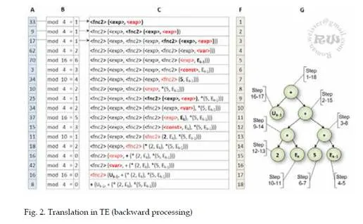
Transplant Evolution (TE) was inspired by biological transplantation. It is an analogy to the transplant  surgery  of  organs.  Every  transplanted  organ  was  created  by  DNA  information but some parts of an ill body can be replaced by a new organ from the database of organs. The description parts of individual (organs) in the database are not stored on the level DNA (genotype).  In  Transplant  Evolution  (TE)  every  individual  part  (organ)  is  created  by  the translation   of   grammar   rules   similar   to   Grammatical   Evolution   (GE),   but   Transplant Evolution (TE) does not store the genotype and the grammatical rules are chosen randomly. The newly created structure is stored only as a tree. This is like Genetic Programming (GP). The   Transplant   Evolution   algorithm   (TE)   combines   the   best   properties   of   Genetic Programming  (GP)  [2]  and  Grammatical  Evolution  (GE)  [4].  The  Two-Level  Transplant

Evolution  (TLTE)  in  addition  to  that  uses  the  Differential  Evolution  algorithm  (DE).

Optimization   of   the   numerical   parameters   of   general   controllers   in   recurrent   control equations of general controllers is a very difficult problem. We applied the second level of optimization by the Differential Evolution method (DE). The individuals in TE and TLTE are represented only by a phenotype in the shape of an object tree. During the initialization of population and during the creation of these phenotypes, similar methods are used as in GE. In Grammatical Evolution the numerically represented chromosomes are used. The codons of  these  chromosomes  are  used  for  the  selection  of  some  rule  from  a  set  of  rules.  In Transplant  Evolution  the  chromosomes  and  codons  are  not  used,  but  for  the  selection  of some rule from a set of rules randomly generated numbers are used. These numbers are not stored  in  the  individual  chromosome.  The  new  individuals  in  the  population  are  created with  the  use  of  analytic  and  generative  grammar  and  by  using  crossover  and  mutation operators.  These  operators  are  projected  for  work  with  the  phenotype  of  an  individual, similarly  as  in  GP.  Because  the  individuals  of  TE  and  TLTE  are  represented  only  by phenotype,  it  was  possible  to  implement  these?  advanced  methods  in  the  course  of evolution:

•      an effective change of the rules in the course of evolution, without the loss of generated solutions,

•       a  difference  of  probability  in  the  selection  of  rules  from  the  set  of  rules  and  the possibility of this changing

        during the    evolutionary process,

•       the   possibility   of   using   methods   of   direct   reduction   of   the   tree   using   algebraic  operations,

•      there is a possible to insert some solutions into the population, in the form of an inline entry of phenotype

       (for example: Uk-1  + Ek  + Ek-    1  * num),

•       new methods of crossover are possible to use, (for example crossover by linking trees)

•      etc.

Initialization of individual

During  the  initialization,  the  generative  grammar  rules  are  used.  These  rules  are  selected randomly from the set of rules by the following equation:

rule = random(0,maxInt)%rules_count

(1)  Where:  random is  a  pseudo-random  number  generator,  maxInt  is  a  high  number,  %  is  the remainder  operator  (modulus),  and  rules_count  denotes  the  number  of  possible  rules  to transcribe a given non-terminal symbol. The  algorithm  TE  which  is  described  by  equation  1  differs  by  the  way  of  initialization  of individual  in  Grammatical  Evolution  (GE).The  Original  initialization  algorithm  GE  uses forward  processing  of  grammatical  rules.  In  the  Grammatical  Evolution  the  method  of crossover and mutation are made on the genotype level. The phenotype is created by a later translation of this genotype. This way of mutation and crossover does not allow the using of advanced method in crossover and mutation operators, which does not destruct the already created parts of the individual (O’Neill M. and Ryan C., 2003). During the evolution of this algorithm  the  Backward  Processing  of  Rules  (BPR)  arose  (Popelka,  O.,  2007).  The  BPR method uses gene marking. This approach has the hidden knowledge of tree structure. Due to  the  BPR  the  advanced  and  effective  methods  of  crossover  and  mutation  can  be  used. Anyhow  the  BPR  method  has  some  disadvantages.  Due  to  these  disadvantages  the  new

Crossover

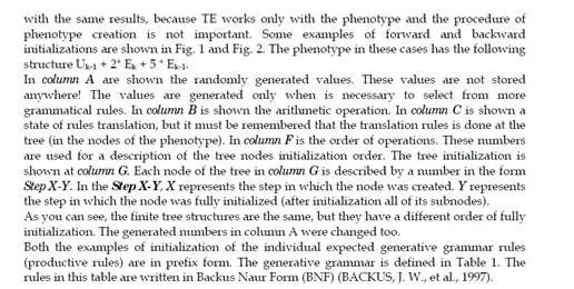
The  crossover  is  a  distinctive  tool  for  genetic  algorithms  and  is  one  of  the  methods  in evolutionary  algorithms  that  are  able  to  acquire  a  new  population  of  individuals.  The crossover is realized in a similar way as in Genetic Programming (GP) [2].

The TE uses three types of crossover. The first type of crossover is named crossover the parts of trees, the second type is named crossover of nodes, and the third type is named crossover by linking  trees.  The  nodes  or  subparts  of  trees  in  the  individuals  for  crossover  are  selected randomly.

In the case of the method crossover of nodes it is neccessary to keep change of the same types of nodes. This request is possible to express by this relationship:

Mutation

Mutation  is  the  second  operator  to  obtain  new  individuals.  This  operator  can  add  new structures,  which  are  not  included  in  the  population  so  far.  Mutation  is  performed  on individuals from the old population. The nodes in the individuals for mutation are selected randomly.  The  mutation  operator  can  be  subdivided  into  two  types.  The  first  type  of mutation   is   non-structural  mutation  and   second   type   is   structural  mutation.   Structural mutation  can  be  divided  into  shortening  structural  mutation  and  extending  structural mutation. The mutation operator uses analytic grammar and generative grammar rules.

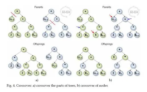
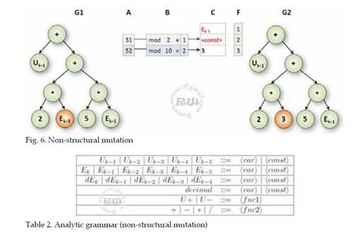
Non-structural mutation does not affect the structure of the already generated individual. In the individual that is selected for mutation, the chosen nodes of the object sub-tree are further  subjected  to  mutation.  The  mutation  will  randomly  change  the  chosen  nodes, whereas the used grammar is respected. For example it means that the mutated node, which is a function of two variables (i.e. + – × ÷) cannot be changed by the node representing the function of one variable (unary minus, etc.) or only a variable (Ek, etc.), etc. See Fig. 6.

The selected node in the tree G1 is marked by an orange color (or a different level of gray).The tree after mutation is marked G2 and the mutated node is marked an orange color (or different level of gray) too. The mutation was made by the using of generative and analytic grammar.  The  operations  with  this  grammar  are  marked  in  columns  A,  B,  C,  and  F.  The randomly   generated   value   for   rule   selection   are   shown   in   column   A.   The   modulus operations are shown in column B. The processing of rules is shown in column C.

This example assumes the generative grammar rules in Table 1 and the analytic grammar rules in Table 2.

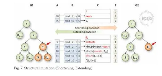
Structural   mutations,   unlike   non-structural   mutations,   affect   the   tree   structure   of individuals.  Changes  of  the  sub-tree  by  extending  or  shortening  its  parts  depend  on  the method   of   structural   mutations.   Structural   mutation   can   be   divided   into   two   types: Structural mutation which is extending an object tree structure and structural mutation which is  shortening a tree structure.  In  the  case  of  the  extending structural mutation,  a  randomly selected node is replaced by a part of the newly created sub-tree that respects the rules of the defined  grammar  (see  Fig.  7).  Conversely  the  shortening  structural  mutation  replaces  a randomly selected node of the tree, including its child nodes, by a node which is described by a terminal symbol (i.e. a variable or a number). This type of mutation can be regarded as a method of indirectly reducing the complexity of the object tree (see Fig. 7).

Architecture

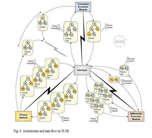
From the implementation viewpoint, the joining of the two evolutionary algorithms is the most   difficult   process.   For   the   best   flexibility   the   interconnecting   of  three   separate computational modules that are join by an interlayer were chosen. The interlayer mediates a communication  among  the  modules  and  prepares  data  in  the  required  form.  With  this implementation  it  is  possible  to  use  each  module  separately  for  another  optimization problem, or similarly to change some module by another module.

Transplant Evolution Module

The transplant Evolution Module (MTE), see Fig. 8 ensures optimization of the structure of controllers. The principle of this algorithm was described in the article TLTE. Its task is to create a population of individuals which uses generative grammar G and analytic grammar G-1.  This  module  can  make  a  numerical  optimization  of  parameters  in  the  structure solutions  too,  but  the  quality  is  not  so  good  as  in  the  case  of  the  two-level  structure. Optimization  of  the  parameters  is  provided  by  the  Differential  Evolution  Module  (MDE). The agent for the communication between these layers is the Interlayer, which is responsible for  preparing  the  data  in  the  desired  form  for  each  module.The  input  parameters  for  the MTE are the generative grammar rules P and the analytic grammar rules P-1, which leads to the  evolution  of  individuals  (solutions).  The  output  parameter  of  the  MTE  is  a  fully optimized solution that includes both the appropriate structure, and its parameters.

Differential Evolution Module

The  Differential  Evolution  Module  (MDE),  see  Fig.  8  ensures  the  optimization  of  abstract parameters in the structure of the individual. The principle function of Differential Evolution (DE) is explained for exiaimi ifple in [4]. This module is activated by the Interlayer, which gives it the vector of variables  num= (num1 ,…,numn )  as one of the input parameters. The number of parameters  of  this  vector  is  equal  to  the  number  of  variables,  which  was  included  in  the structure  of  the  solutions  that  came  from  the  MTE.  The  output  parameter  MDE  is  the optimized vector of parameters that is sent into the Interlayer.

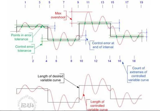
Fitness Module

The  fitness  Module  (FM),  see  Fig.  8,  provides  an  evaluation  of  the  models.  The  model  is some structure of the solutions, including some parameters. This model, together with the controlled system is the input of simulation. For a given controller and controlled system, the  simulation  of  regulation  is  started.  The  quality  of  model  is  included  in  the  fitness function after the finishing of the simulation. The evaluated model is send to the Interlayer.

Interlayer

The Interlayer, see Fig. 8 is the most important part in the whole architecture of Two-Level architecture.   The   Interlayer   is   the   main   module,   which   holds   instances   of   all   the computational  modules.  The  interlayer provides  communication  among  the  computational modules through the communication interface. This module contains the knowledge about the strategy of optimization so this means what to be optimized and how to optimize it. The interlayer controls the parameters of all the computational modules (MTE, MDE, and FM), for  example:  size  of  populations  TE  or  DE,  number  of  generations,  type  of  selection methods,  set of  probability  of  crossover  and  mutation,  etc.  The  interlayer  makes  the communication with an Output Module (OM). The OM is a graphical output, which shows the  evolution  outputs,  simulation  of  control  outputs,  etc.  The  most  important  task  of  the interlayer  is  data  preparation  in  the  correct  form  during  the  communication  among  the computational  modules,  for  example  during  the  request  for  fitness  evaluation,  see  Fig.  8. From this perspective, the tasks can be divided as follows:

•      To  create  the  vector  of  symbolic  variables  for  MDE  during  the  communication  with MTE.

•      The abstract variables will be set by concrete optimized parameters in abstract variables after the finishing of the optimization.

•       To  send  a  full  model  of  the  solution  (structure  +  parameters)  to  the  FM,  during  the request of the MTE for the calculation of the    quality of an individual, which does not include any abstract parameter.

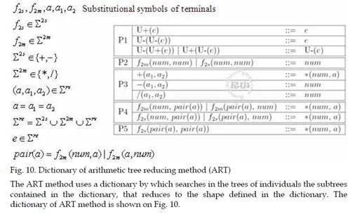
Arithmetic tree reducing

By penalizing the part of the individual fitness which contains  a complex object tree,   the method of targeted shortening structural mutation of individual, or   the direct shortening of the tree using algebraic adjustments – Algebraic Reducing Tree (ART).

•      By penalizing the part of the individual fitness which contains a complex object tree,

•       Method of targeted shortening structural mutation of individual,

•      The direct shortening of the tree using algebraic adjustments – Algebraic Reducing Tree (ART).

The last-mentioned method can be realized by the TE, where all of the individuals do not contain the genotype, and then a change in the phenotype is not affected by treatment with the  genotype.  The  realization  of  the  above  mentioned  problem  with  an  individual,  which uses  the  genotype  would  be  in  this  case  very  difficult.  This  new  method  is  based  on  the algebraic  arrangement  of  the  tree  features  that  are  intended  to  reduce  the  number  of functional blocks in the body of individuals (such as repeating blocks “unary minus”, etc.).

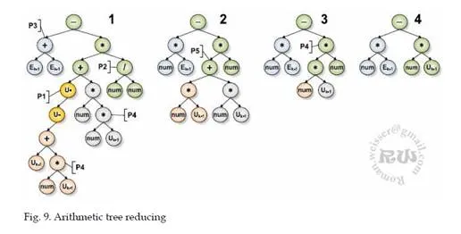
In view of the object tree complexity of the individual and also for the subsequent crossover it is preferable to have a function in the form of  x = 3 × a, rather than x = a + a + a, or more generally x = n × A. Another example is the shortening of the function x = – (- a), where the form  x = a  is preferable (it is removing the redundant marks in the object tree individual). The introduction of algebraic modifications of the individual phenotype leads to a shorter result of the optimal solution and consequently to a shorter presentation of the individual and the shortening of the time of calculation of the function that is represented in the object tree  and  also  to  finding  optimal  solutions  faster  because  of  the  higher  probability  of crossover in the suitable points with a higher probability to produce meaningful solutions. The essential difference stems from the use of the direct contraction of trees, which leads to a significantly shorter resulting structure than without using this method. The arithmetic tree reducing method is shown on Fig. 9. The tree on the beginning of the process  of  ART  is  shown  under  the  number  1,  the  resulting  tree  after  the  use  of  ART  is shown under number 4.