Fluid kinematics – Mechanical Engineering

Kinematics is defined as the geometry of the motion.

Fluid kinematics defines the motion of the fluids and its significance without taking into account of the nature of forces that cause motion.

Kinematics is divided into three main features:

Improvement of methods and tools for recitation and identifying the motion of fluids.
Determination of the conditions for the kinematic option of fluid motions
Classification of different kinds of motions and related distortion rates of any fluid component.

Scalar and vector Sector:

Scalar is a quantity which can be expressed by a particular number represents its magnitude.

Examples: Temperature, mass and density

Scalar sector:

In a region if every point of the scalar functions has a defined value, then that region is known as the scalar sector.

Example: In a rod temperature must be distributed.

Vector

Vector is a quantity which can be expressed in both the direction and the magnitude.

Examples: Displacement, velocity and force.

Vector Sector:

In a region if every point of the vector functions has a defined value. Then that region is known as the vector sector.

Example: velocity of the flowing fluid

Flow sector:

The area in which the flow elements such as pressure, velocity etc., which are to be defined at every point of an instant of time is known as flow sector.

Flow sectors are identified by the velocity observed at different areas in that particular region, at various times factors.

Various types of fluid motions:

Fluid motions are divided into two types they are

Lagrangian method
Eulerian Method

Lagrangian method

Lagrangian methods is used for single fluid particles

Advantages of Lagrangian method:

History of the method can be traced with the help of the motion and trajectory of the fluid particles.
From the beginning of the method the particles are traced throughout the motion, where exchange of mass is essential.

Disadvantages of Lagranigian method:

For practical applications this method is rarely used.

Eulerian Method

Eulerian method is developed by Leonhard Euler

This method is used for particular section or point.

Relation between the Lagrangian and Eulerian concept

For Eulerian, we can written as

$\frac{dx}{dt}=u(x,y,z,t)$
$\frac{dy}{dt}=v(x,y,z,t)$
$\frac{dz}{dt}=w(x,y,z,t)$

From Lagrangian, we can written as

From the Eularian method the Lagranigian method are derived.

Variation of flow parameters:

Steady flow:

At a point where the flow characteristics, and fluid parameters do not change with respect to the time, such a flow is referred as steady flow.

According to the Eulerian method steady flow is defined as

\vec{V}=V(\vec S) \:\: and \:\: \vec a=a (\vec S)

Unsteady flow:

In the unsteady flow the flow characteristics and fluid parameters are changed with the time.

Uniform flow:

At any instant of time the velocity vectors flow uniform and they do not change point to point with time, which called as uniform flow.

Non – Uniform flow:

At any instant of time the velocity vector varies from point to point of time is known as the non – uniform flow.

This flow is applicable for the velocity only.

Turbulent flow:

The particles that have the random and erratic movement, intermixing with the adjacent layers is known as the turbulent flow.

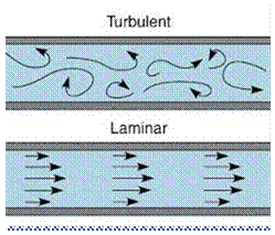
Laminar Flow:

When the particles move in layers sliding smoothly over the adjacent layer are known as laminar flow.

Streak line:

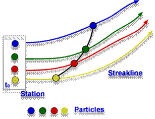
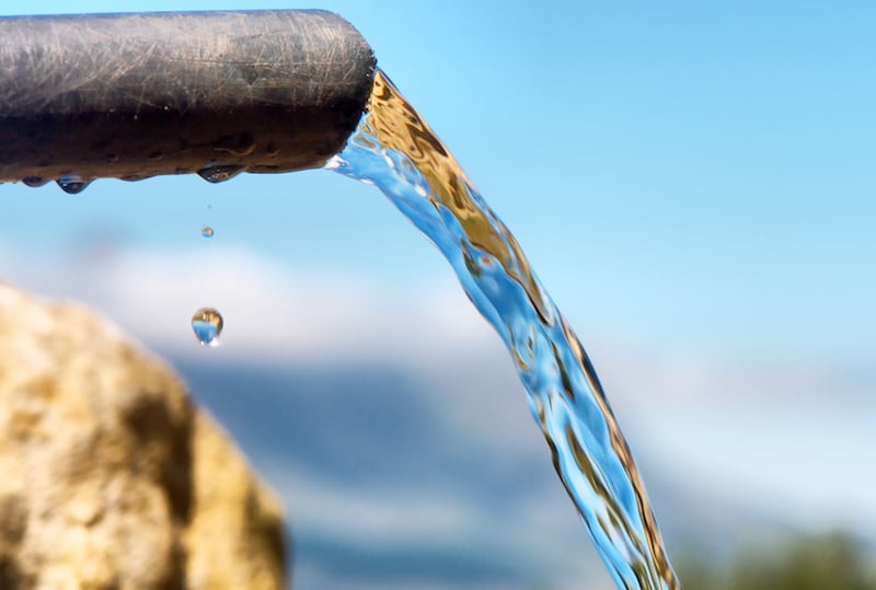
Streak lines are the locus of the points. In the past all the particles that always passes through a specific spatial point. Dye steadily inserted into the fluid at a static point spreads along a streak line.

Mathematical Description:

Streak lines are defined as:

$ \vec {u_P}”> Is the velocity of the particle and P is the location at <img bv-data-src=$

During motion path line is a curve traced by a single fluid particle

Mathematical Description:

Path line is defined as:

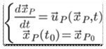
</p><br /><br /><br /> <p>\left\{\begin{matrix}<br /><br /><br /><br /> \frac{d\vec x_P}{dt}=\vec u_P(\vec x_P,t) \\<br /><br /><br /><br /> \vec x_P(t_0)=\vec x_{P_0}<br /><br /><br /><br /> \end{matrix}

P indicates the motion of a fluid particle. At the point $ \vec {x_P}”> the curve must be parallel to the flow of the velocity vector <img bv-data-src=$ .The velocity vector is calculated at the position of the particle $ \vec {x_P}”> at that time t. Streamline: <figure class=$

Streamline is defined as an imaginary line which is drawn in a flow field, such as a tangent drawn at any point. On that line it represents the direction of the velocity vector at that point.

There is no velocity component normal to the stream lines.

Mathematical description:

Streamline is defined as:

\frac{d\vec x_S}{ds}\times \vec u(\vec x_S)=0

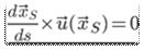
where,

x= vector cross product and

$\vec x_S(S)$ = parametric representation of single streamline at single moment in time.

Velocity of the components $\vec u$ =(u,v,w) and stream lines are expressed as $\vec {x_s}=(x_s,y_s,z_s)$ we assume it as

Related Posts