Here at CAE Associates, we get a lot of different questions from our clients during training classes and technical support. One of the more common questions is about finite element mesh quality.  Finite element preprocessors have come a long way over the years, to the point where users with minimal training can create meshes that appear “good”.  But, how can you really know if the mesh is good enough for your analysis?  Meshes that are “good enough” are ones that produce results with an acceptable level of accuracy, assuming that all other inputs to the model are accurate.  Mesh density is a significant metric used to control accuracy (element type and shape also affect accuracy).  Assuming no singularities are present, a high-density mesh will produce results with high accuracy.  However, if a mesh is too dense, it will require a large amount of computer memory and long run times, especially for multiple-iteration runs that are typical of nonlinear and transient analyses.

One of the ways to evaluate the quality of your mesh (and a model overall) is to compare results to test data or to theoretical values.  Unfortunately, test data and theoretical results are often not available.  So, other means of evaluating mesh quality are needed.  These include mesh refinement and interpretations of results discontinuities.

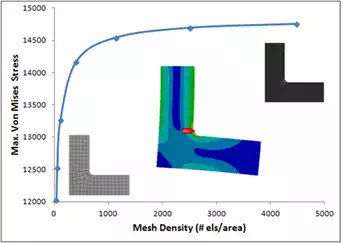
The most fundamental and accurate method for evaluating mesh quality is to refine the mesh until a critical result, such as the maximum stress in a specific location converges (i.e. it doesn’t change significantly with each refinement).   An example is shown in Figure 1, where a 2D bracket model is constrained at its top end and subjected to a shear load at the edge on the lower right.  This generates a peak stress in the fillet, as shown.  The curve shows that as the mesh density increases, the peak stress in the fillet increases.  Ultimately, increasing the mesh density further produces only minor increases in peak stress.  In this case, an increase from 1134 elements per unit area to 4483 elements per unit area yields only a 1.5% increase in stress.

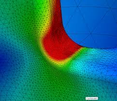
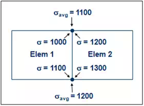
The problem with this method is that it requires multiple remeshing and re-solving operations.  While this method is fine for simple models, it can be very time-consuming for complex models.  Another option is to evaluate the magnitude of stress discontinuity between adjacent elements in the critical region.  In most cases, the finite element method computes stresses directly at interior locations of the element (Gauss points) and extrapolates them to the nodes on the element boundaries.  While it is common to view these stresses as average values, the reality is that each element calculates different stresses at shared nodes, as illustrated in Figure 2.  The degree of stress discontinuity decreases with improving mesh quality, so this metric can be used to gauge mesh quality.

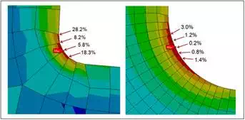
Building on the earlier example, Figure 3 shows the relative difference in unaveraged stresses at shared nodes in the fillet region of the bracket.  These percentages were calculated by taking the difference in unaveraged stresses and dividing them by the nodal averaged stress.  The finer mesh shown on the right generates much lower relative differences in the fillet which indicates that this mesh is considerably more accurate.  The percentage difference also indicates the degree of potential error in the solution.  While other error measures can be used, they are generally all based on the difference in the critical results between adjacent elements at their shared nodes.

It should be noted that it is quite common and perfectly acceptable to have high relative stress differences in regions farther from the critical locations in your model where stresses are lower.  This is often the case because these regions are not meshed at a high density and sometimes because they contain singularities.  However, it is up to the analyst to determine if a high degree of accuracy is important in a given region and, if it is, to evaluate the quality of the mesh in that region.  Mesh quality is extremely important to overall model accuracy for your FEA consulting projects and can ultimately mean the difference between predicting that a design will or will not fail.

Planar Microstrip Patch Antenna Design in Free Space

There are a variety of wearable antennas, such as planar dipoles, monopoles, planar inverted-Fs and microstrip patches. Microstrip antennas are planar and can be easily made onto a printed circuit board (PCB), which makes them a practical antenna type due to their low cost and easy fabrication. Figure 1 shows the structure of a planar microstrip inset fed patch antenna, where the resonant frequency is related to the width W1 and length L1 of the patch, the substrate thickness h and permittivity εr of the dielectric. The antenna is printed on a dielectric substrate with permittivity εr = 3.38 and h = 1.254mm. The antenna consists of an inset patch and a 50 Ohm microstrip feed line on the top side of the substrate, and a ground plane of 1mm thickness on its bottom side [1].

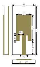
Figure 1 – Planar Inset Fed Microstrip Patch Antenna Structur

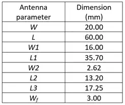
Table 1 – Antenna dimensions

 The ANSYS Electronics Desktop is used to optimise the antenna dimensions so that the antenna resonates at around 2.4 GHz. Figure 2 shows the antenna model in the ANSYS Electronics Desktop. Figure 3 shows the simulated return loss of the optimised antenna in free space, and Table 1 lists its dimensions.

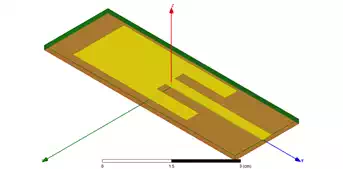
Figure 2 – Planar Inset Fed Microstrip Patch Antenna Model using the ANSYS Electronics Desktop

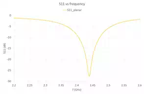
Figure 3 – Planar Inset Fed Microstrip Patch Antenna Return Loss

Wearable Non-planar Conformal Antenna Structure

The proposed wearable antennas are designed to be worn on the exterior body and outer garments or tactical vests operating in the 2.4GHz wireless networking band. Let us suppose these antennas are to be worn on a wrist. Three different cylinders with radius R=5, 7.5 and 10cm were chosen to bend the antennas, corresponding to typical sizes of the human wrist. Figure 4 shows the conformal antenna models in the ANSYS Electronics Desktop, and Figure 5 shows the return loss of conformal antenna models.

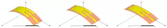
Figure 4 – Cylindrically Curved Structures of radii 5cm, 7.5cm and 10cm

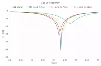
Figure 5 – Return Loss of Cylindrically Curved Structures of radii 5cm, 7.5cm and 10cm

From Figure 5, it is seen that the resonance frequencies changed from 2.44GHz (planar) to 2.47GHz (R=5cm), 2.42GHz (R=7.5cm) and 2.43GHz (R=10cm). This will give practical design guideline when choosing the operating frequency of conformed antennas.

Conformal Antenna Structure Worn on Wrist

The antenna performance while in close proximity to the human body is our main concern. The ANSYS Electronics Desktop provides a human body model library which makes it convenient to add a human body 3D component. Figure 6 shows the model of a conformal antenna worn on wrist in the ANSYS Electronics Desktop.

Figure 7 shows the return loss variation with placing conformal antennas on human wrist. The dotted lines represent conformal antennas in free space, while the solid lines represent those worn on wrist. With antennas closer to human body, the resonance damps a little, and the resonant frequency has minor shift. Figure 8 shows the gain pattern change at 2.4GHz after placing the conformal antenna of curving radius 5cm on wrist, letting the antenna centre placed on the original point of coordinate system. To investigate the gain pattern in more details, Figure 9 shows the gain pattern with the antenna overlay. After placing the antenna on human wrist, the antenna radiation is more focused in the positive half space (z>0), since in the negative half space (z<0) the radiation is mostly blocked by the wrist beneath the antenna.

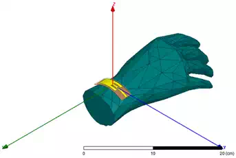
Figure 6 – Conformal Antenna Structure Worn on Wrist

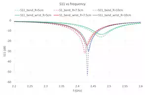
Figure 7 – Return Loss of Cylindrically Curved Structures of radii 5cm, 7.5cm and 10cm before and after being placed on wrist

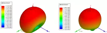
Figure 8 – Gain of Cylindrically Curved Structures of radii 5cm before and after being placed on wrist

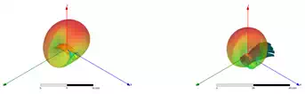
Figure 9 – Gain of Cylindrically Curved Structures of radii 5cm before and after being placed on wrist with antenna overlay

This example demonstrates the power of the ANSYS Electronics Desktop for efficiently designing wearable antennas and simulating the impact of real world scenarios. The ANSYS Electronics Desktop provides an accurate calculation and visual elaboration on the antenna performance, such as return loss, resonant frequency and radiation performance. It helps us to reach the design target by not only optimising the performance within a variety of variables, but also predicting the behaviour of whole system.

In conclusion, the ANSYS Electronics Desktop provides a highly efficient solution for high fidelity antenna design and optimisation.