The fractional calculus is a branch of mathematics that attracted attention since G.W. Leibnitz proposed it in the seventeenth century. However, the researchers were not attracted to this area because of the lack of applications and analytical results of the fractional calculus.On the contrary, the fractional calculus currently attracts the attention of a large number of scientists for their applications in different fields of science, engineering, chemistry, and so on.This chapter presents the design of a fractional order nonlinear identifier modeled by a dynamic neural network of fractional order.Although PID controllers are introduced long time ago, they are widely used in industry because of their advantages such as low price, design simplicity, and suitable performance. While three parameters of design including proportional (Kp), integral (Ki), and derivative (Kd) are available in PID controllers, two more parameters exist in FOPID controllers for adjustment.
These parameters are integral fractional order and derivative fractional order. In comparison with PID controllers, FOPID controllers have more flexible design that results in more precise adjustment of closed‐loop system. FOPID controllers are defined by FO differential equations. It is possible to tune frequency response of the control system by expanding integral and derivative terms of the PID controller to fractional order case. This characteristic feature results in a more robust design of control system, but it is not easily possible. According to nonlinearity, uncertainty, and confusion behaviors of robot arms, they are highly recommended for experimenting designs of control systems. Despite nonlinear behavior of robot arm, it is demonstrable that a linear proportional derivative controller can stabilize the system using Lyapunov. But, classic PD controller itself cannot control robot to reach suitable condition. Several papers and wide researches in optimizing performance of the robot manipulator show the importance of this issue.
There are several ways of defining the derivative and fractional integral, for example, the derivative of Grunwald‐Letnikov given by Eq. (1)
where [.] is a flooring operator, while the RL definition is given by:
For (n−1<α<n)(n−1<α<n), Γ(x)Γ(x) is the well‐known Euler’s Gamma function.Similarly, the notation used in ordinary differential equations, we will use the following notation, Eq. (3), when we are referring to the fractional order differential equations where αk∈R+αk∈R+.which is:
The Caputo’s definition can be written as
| aDαtf(t)=1Γ(α−n)∫atf(n)(τ)(t−τ)α−n+1dτaDtαf(t)=1Γ(α−n)∫atf(n)(τ)(t−τ)α−n+1dτ | (4) |
For
Trajectory tracking, synchronization, and control of linear and nonlinear systems are a very important problem in science and control engineering. In this chapter, we will extend these concepts to force the nonlinear system (plant) to follow any linear and nonlinear reference signals generated by fractional order differential equations.
The proposed adaptive control scheme is composed of a recurrent neural identifier and a controller (Figure 1).
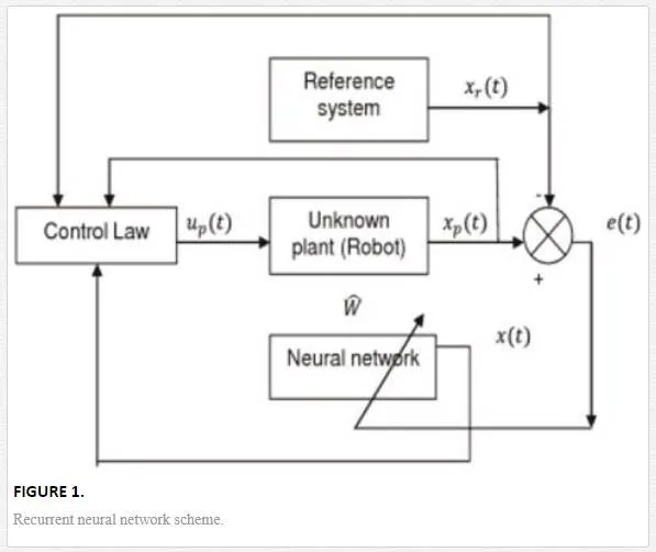
We use the above scheme to model the unknown nonlinear system by means of a dynamic recurrent neural network of adaptable weights; the above is modeled by differential equations of fractional order. Also, the scheme allows us to determine the control actions, the error of approach of trajectories, as well as the laws of adaptation of adaptive weights and the interconnection of such systems.
Modelling of the plant
The nonlinear system (Eq. (5)) is forced to follow a reference signal:
| aDαtxp=Fp(xp,u)≜fp(xp)+ gp(xp)upxp, fp.∈Rn, u∈Rm, gp∈Rnxn.aDtαxp=Fp(xp,u)≜fp(xp)+ gp(xp)upxp, fp.∈Rn, u∈Rm, gp∈Rnxn. | (5) |
The differential equation will be modeled by:
aDαtxp=A(x)+W*Γz(x)+Ωu.aDtαxp=A(x)+W*Γz(x)+Ωu.
The tracking error between these two systems:
| wper=x−xpwper=x−xp | (6) |
We use the next hypotheses.
| aDαtwper=−kwperaDtαwper=−kwper | (7) |
In this research, we will use k=1k=1, so that, Eq. (6), aDαtwper=aDαtx−aDαtxpaDtαwper=aDtαx−aDtαxp,; so
aDαtxp= aDαtx+wperaDtαxp= aDtαx+wper
The nonlinear system is [1]:
| aDαtxp=aDαtx+wper=A(x)+W*Γz(x)+wper+ΩuaDtαxp=aDtαx+wper=A(x)+W*Γz(x)+wper+Ωu | (8) |
Where the W*W* is the matrix weights.
 Tracking error problem
In this part, we will analyze the trajectory tracking problem generated by
| aDαtxr=fr(xr,ur), wr, xr∈RnaDtαxr=fr(xr,ur), wr, xr∈Rn | (9) |
Are the state space vector, input vector, and frfr, is a nonlinear vectorial function.
To achieve our goal of trajectory tracking, we propose
| e=xp−xre=xp−xr | (10) |
The time derivative of the error is:
| aDαte=aDαtxp−aDαtxr=A(x)+W*Γz(x)+wper+Ωu−fr(xr,ur)aDtαe=aDtαxp−aDtαxr=A(x)+W*Γz(x)+wper+Ωu−fr(xr,ur) | (11) |
The Eq. (11) can be rewritten as follows, adding and subtracting the next terms WˆΓz(xr)W^Γz(xr), αr(t,Wˆ)αr(t,W^), AeAe and wper=x−xpwper=x−xp,; then,
The unknown plant will follow the fractional order reference signal, if:
Axr+WˆΓz(xr)+xr−xp+Ωαr(t,Wˆ)=fr(xr,ur)Axr+W^Γz(xr)+xr−xp+Ωαr(t,W^)=fr(xr,ur), where
| aDαte=Ae+W*Γz(x)−WˆΓz(xr)−Ae+(A+I)(x−xr)+Ω(u−αr(t,Wˆ))aDtαe=Ae+W*Γz(x)−W^Γz(xr)−Ae+(A+I)(x−xr)+Ω(u−αr(t,W^)) | (14) |
Now, WˆW^ is part of the approach, given by W*W*. The Eq. (14) can be expressed as Eq. (15), adding and subtracting the term WˆΓz(x)W^Γz(x) and if Γz(x)=Γ(z(x)−z(xr))Γz(x)=Γ(z(x)−z(xr))
| aDαte=Ae+(W*−Wˆ)Γz(x)+WˆΓ(z(x)−z(xr))+(A+I)(x−xr)−Ae+Ω(u−αr(t,Wˆ))aDtαe=Ae+(W*−W^)Γz(x)+W^Γ(z(x)−z(xr))+(A+I)(x−xr)−Ae+Ω(u−αr(t,W^)) | (15) |
If
And by replacing Eq. (16) in Eq. (15), we have:
aDαte=Ae+W∼Γz(x)+WˆΓ(z(x)−z(xr))+(A+I)(x−xr)−Ae+Ωu∼aDtαe=Ae+W∼Γz(x)+W^Γ(z(x)−z(xr))+(A+I)(x−xr)−Ae+Ωu∼
| aDαte=Ae+W∼Γz(x)+WˆΓ(z(x)−z(xp)+z(xp)−z(xr))+(A+I)(x−xp+xp−xr)−Ae+Ωu∼aDtαe=Ae+W∼Γz(x)+W^Γ(z(x)−z(xp)+z(xp)−z(xr))+(A+I)(x−xp+xp−xr)−Ae+Ωu∼ | (17) |
And:
So, the result for Ωu1Ωu1 is
and Eq. (17) is simplified:
aDαte=Ae+W∼Γz(x)+WˆΓ(z(xp)−z(xr))+(A+I)(xp−xr)−Ae+Ωu∼aDtαe=Ae+W∼Γz(x)+W^Γ(z(xp)−z(xr))+(A+I)(xp−xr)−Ae+Ωu∼
Taking into account that e=xp−xre=xp−xr, the equation for aDαteaDtαe is
aDαte=(A+I)e+WËœΓz(x)+WˆΓ(z(e+xr)−z(xr))+Ωu2=(A+I)e+W∼σ(x)+Wˆ(σ(e+xr)−σ(xr))+Ωu2aDtαe=(A+I)e+WËœΓz(x)+W^Γ(z(e+xr)−z(xr))+Ωu2=(A+I)e+W∼σ(x)+W^(σ(e+xr)−σ(xr))+Ωu2
If φ(e)=(σ(e+xr)−σ(xr))φ(e)=(σ(e+xr)−σ(xr)), then
Now, the problem is to find the control law Ωu2Ωu2, in which it stabilizes to the system Eq. (20). We will obtain the control law using the fractional order Lyapunov methodology.
Asymptotic stability of the approximation error
From Eq. (20), we consider the stability of the tracking error, for which we first observe that (e,Wˆ)=0(e,W^)=0, is an equilibrium state of dynamical system from Eq. (20), and we consider a particular case when A=−λIA=−λI ,λ>0λ>0
For such stability analysis of the trajectory tracking (Eq. (20)), we propose the following FOPID control law [2]:
Our objective is to find KpKp, KiKi, KvKv,WˆW^, L2φzLφz2, and this guarantees that the tracking error given by Eq. (20) is asymptotically stable, for which we will later propose a Lyapunov function, with γ>0γ>0 ; this control law (Eq. (21)) is similar to [3].
A FOPID controller, also known as a PIλDαPIλDα controller, takes on the form [4]:
u(t)=Kpe(t)+KiaD−λte(t)+KdaDαte(t)u(t)=Kpe(t)+KiaDt−λe(t)+KdaDtαe(t)
where λλ and αα are the fractional orders of the controller and e(t)e(t) is the system error, where λ=αλ=α. Note that the system error e(t)e(t) replaces the general function f(t)f(t).
We will show that the feedback system is asymptotically stable. Replacing Eq. (21) in Eq. (20), we have
aDαte=(A+I)e+W∼σ(x)+Wˆφ(e)+Kpe+KiaD−αte+KvaDαte−γ(12+12∥∥∥Wˆ∥∥∥2L2φ)eaDtαe=(A+I)e+W∼σ(x)+W^φ(e)+Kpe+KiaDt−αe+KvaDtαe−γ(12+12‖W^‖2Lφ2)e, then
(1−Kv)aDαte=(A+I)e+W∼σ(x)+Wˆφ(e)+Kpe+KiaD−αte−γ(12+12∥∥∥Wˆ∥∥∥2L2φ)e(1−Kv)aDtαe=(A+I)e+W∼σ(x)+W^φ(e)+Kpe+KiaDt−αe−γ(12+12‖W^‖2Lφ2)e. If
a=(1−Kv)a=(1−Kv), then
| aDαte=1a(A+I)e+1aW∼σ(x)+1aWˆφ(e)+1aKpe+1aKiaD−αte−γa(12+12Wˆ2L2φ)eaDtαe=1a(A+I)e+1aW∼σ(x)+1aW^φ(e)+1aKpe+1aKiaDt−αe−γa(12+12W^2Lφ2)e | (22) |
| aDαte=−1a(λ−1+Kp)e+1aW∼σ(x)+1aWˆφ(e)+1aKiaD−αte−γa(12+12Wˆ2L2φ)eaDtαe=−1a(λ−1+Kp)e+1aW∼σ(x)+1aW^φ(e)+1aKiaDt−αe−γa(12+12W^2Lφ2)e | (23) |
And if w=1aKiaD−αtew=1aKiaDt−αe, then aDαtw=1aKie(t)aDtαw=1aKie(t) [5]; then, we rewrite Eq. (23) as:
| aDαte=−1a(λ−1+Kp)e+1aW∼σ(x)+1aWˆφ(e)+w−γa(12+12Wˆ2L2φ)eaDtαe=−1a(λ−1+Kp)e+1aW∼σ(x)+1aW^φ(e)+w−γa(12+12W^2Lφ2)e | (24) |
We will show that the new state (e,w)T(e,w)T is asymptotically stable and the equilibrium point is (e,w)T=(0,0)T(e,w)T=(0,0)T, when W∼σ(xr)=0W∼σ(xr)=0, as an external disturbance.
Let VV be, the next candidate Lyapunov function as [6]:
The fractional order time derivative of Eq. (25) along with the trajectories of Eq. (24) is
| aDαtV=eT(−1a(λ−1+Kp)e+1aW∼σ(x)+1aWˆφ(e)+w−γa(12+12Wˆ2L2φ)e)+1aW∼TKie+1atr{aDαt W∼TW∼}aDtαV=eT(−1a(λ−1+Kp)e+1aW∼σ(x)+1aW^φ(e)+w−γa(12+12W^2Lφ2)e)+1aW∼TKie+1atr{aDtα W∼TW∼} | (27) |
In this part, we select the next learning law from the neural network weights as in [7] and [8]:
Then, Eq. (27) is reduced to
| aDαtV=−1a(λ−1+Kp)eTe+eTaWˆφ(e)+(1+Kia)eTw−γa(12+12∥∥∥Wˆ∥∥∥2L2φ)eTeaDtαV=−1a(λ−1+Kp)eTe+eTaW^φ(e)+(1+Kia)eTw−γa(12+12‖W^‖2Lφ2)eTe | (29) |
Next, lets consider the following inequality proved in [9]
which holds for all matrices X,Y∈RnxkX,Y∈Rnxk and Λ∈RnxnΛ∈Rnxn with Λ=ΛT>0Λ=ΛT>0. Applying (30) with Λ=IΛ=I to the term eTaWˆφ(e)eTaW^φ(e) from Eq. (29), where
eTWˆφ(e)≤12∥∥∥e∥∥∥2+12L2φ∥∥∥Wˆ∥∥∥2e2=12(1+L2φ∥∥Wˆ∥∥2)∥∥∥e∥∥∥2eTW^φ(e)≤12‖e‖2+12Lφ2‖W^‖2e2=12(1+Lφ2‖W^‖2)‖e‖2
we get
| aDαtV≤−1a(λ−1+Kp)eTe+1a(eTe2+12∥∥Wˆ∥∥2L2φ)eTe+(1+Kia)eTw−γa(12+12∥∥∥Wˆ∥∥∥2L2φ)eTeaDtαV≤−1a(λ−1+Kp)eTe+1a(eTe2+12‖W^‖2Lφ2)eTe+(1+Kia)eTw−γa(12+12‖W^‖2Lφ2)eTe | (31) |
Here, we select (1+Kia)=0(1+Kia)=0 and Kv=Ki+1Kv=Ki+1, with Kv≥0Kv≥0 then Ki≥−1Ki≥−1, with this selection of the parameters from Eq. (31) is reduced to:
Of the previous inequality, Eq. (32), we need that the fractional order Lyapunov derivative, aDαtV≤0aDtαV≤0, to ensure that the trajectory tracking error is asymptotically stable, that is, limt→∞e(t)=0limt→∞e(t)=0, which means that the nonlinear system follows the reference signal.
To achieve this purpose, we select:
λ−1+Kp>0,a>0,(γ−1)>0,aDαtV≤0,∀ e, w, Wˆ≠0,e≠0λ−1+Kp>0,a>0,(γ−1)>0,aDtαV≤0,∀ e, w, W^≠0,e≠0
With the above Eq. (32), the control law that guarantees asymptotic stability of the tracking error is given by Eq. (33)
Theorem: The control laws (Eq. (33)) and the adaptive weights (Eq. (28)) ensure that the trajectory tracking error between the fractional nonlinear system (Eq. (8)) and the fractional reference signal (Eq. (9)) satisfies limt→∞e(t)=0limt→∞e(t)=0
Remark 2: From Eq. (32), we have
aDαtV≤−1a(λ−1+Kp)eTe−(γ−1)a(12+12∥∥∥Wˆ∥∥∥2L2φ)eTe<0aDtαV≤−1a(λ−1+Kp)eTe−(γ−1)a(12+12‖W^‖2Lφ2)eTe<0, ∀ e≠0, ∀ Wˆ∀ e≠0, ∀ W^, where VV is decreasing and bounded from below by V(0)V(0), and:
V=12(eT,wT)(e,w)T+12atr{W∼TW∼}V=12(eT,wT)(e,w)T+12atr{W∼TW∼},; then we conclude that e, W∼∈L1e, W∼∈L1; this means that the weights remain bounded.
Simulation
The manipulator used for simulation is a two revolute joined robot (planar elbow manipulator), as shown in Figure 2.
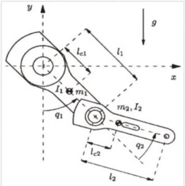
The dynamics of the robot is established by [10, 11], Mij(q), i, j=1,2Mij(q), i, j=1,2 of the inertia matrix M(q)M(q) as
The terms containing αα indicate the additional terms resulting from the fractional order model and the right‐hand sides denote the generalized force terms resulting from the forcing functions, and there is a specific set of values for Q1Q1 and Q2Q2 for each case.
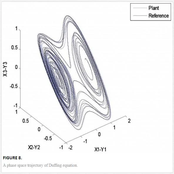
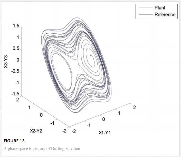
With the end of supporting the effectiveness of the proposed controller, we have used a Duffing equation.
The fractional order neural network is modelling by the differential equation:
aDαtxp=A(x)+W*Γz(x)+ΩuaDtαxp=A(x)+W*Γz(x)+Ωu, with A=−λI,I∈R4x4A=−λI,I∈R4x4, and λ=20λ=20, W*W* is estimated using the learning law given in Eq. (28).
Γz(x)=(tanh(x1), tanh(x2),…,tanh(xn))TΓz(x)=(tanh(x1), tanh(x2),…,tanh(xn))T, Ω=(00 1000 01)TΩ=(00 1000 01)T and the uu is calculated using Eq. (33). The plant is stated in [3] and [13], and it is given by:
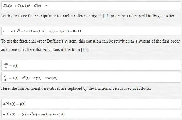
where αα is the fractional orders and α, δ, ωα, δ, ω are the system parameters.
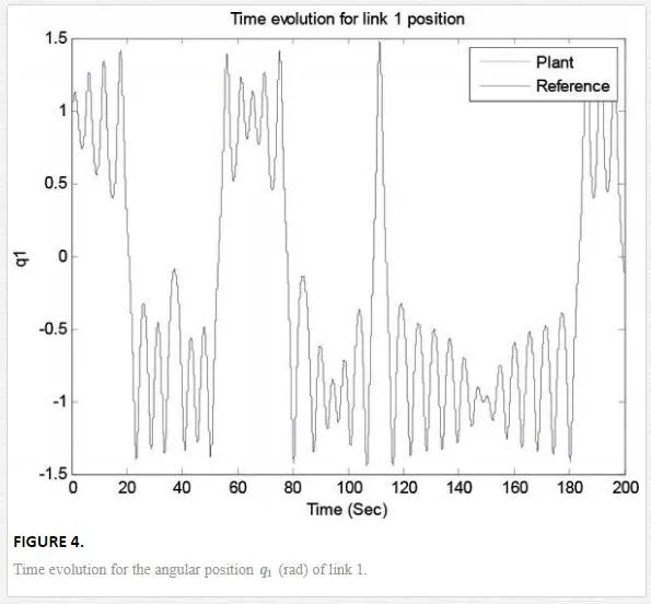
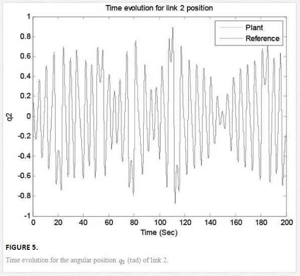
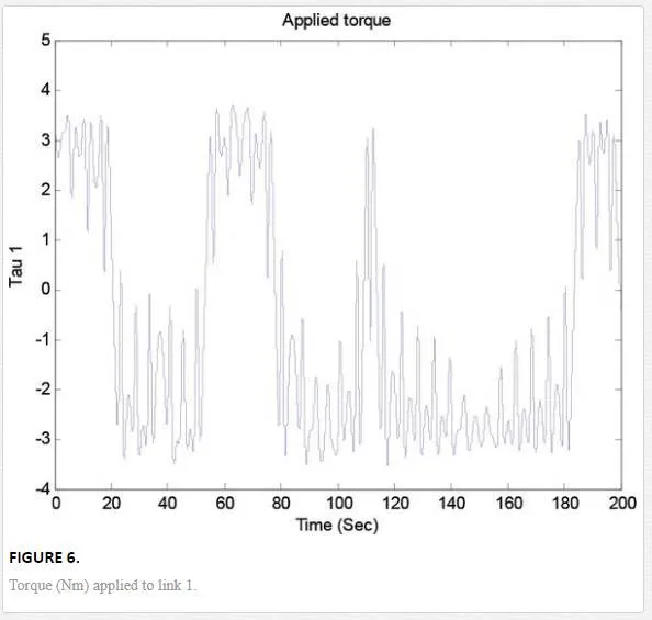
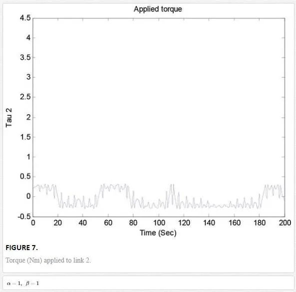
Illustrated, the response in the time, angular position and torque applied to the fractional nonlinear system are shown in Figures 3–7. As can be observed, the trajectory tracking objective is obtained
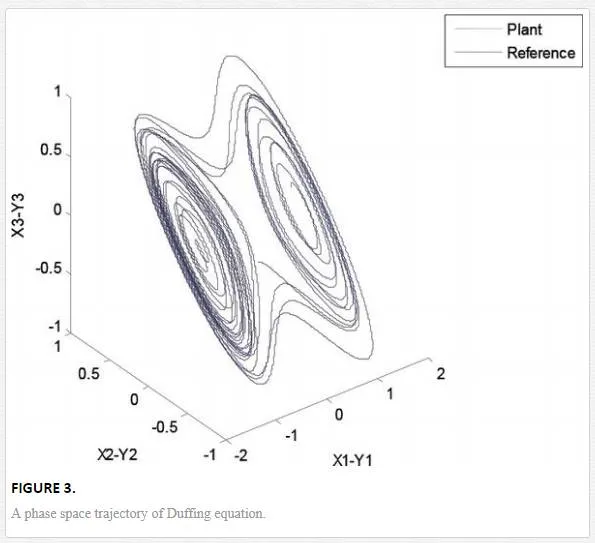
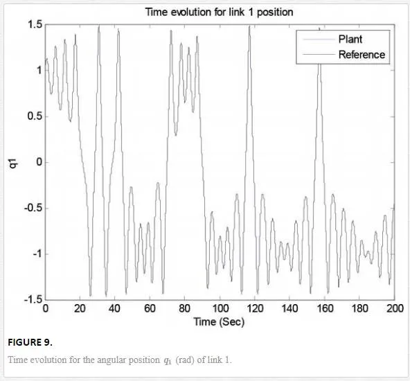
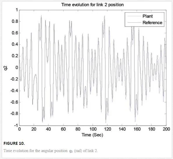
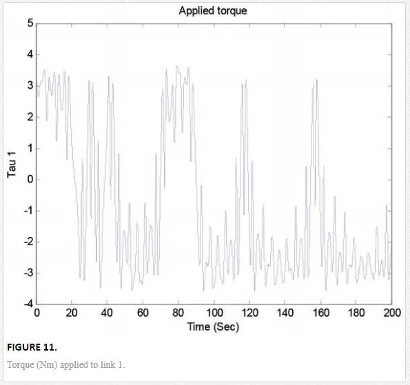
Its phase space trajectory is given in Figure 8, and the time evolution for the position angles and applied torque are shown in Figures 9–12. As can be seen in Figures 9 and 10, the trajectory tracking is successfully obtained where plant and reference signals are the same.
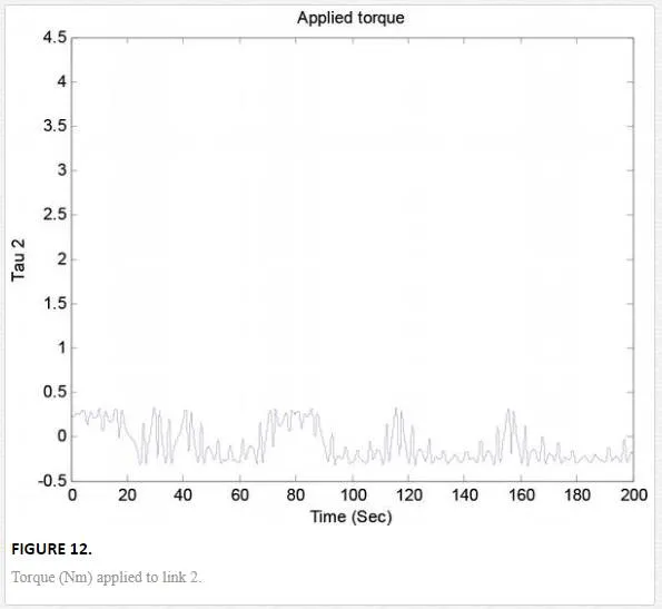

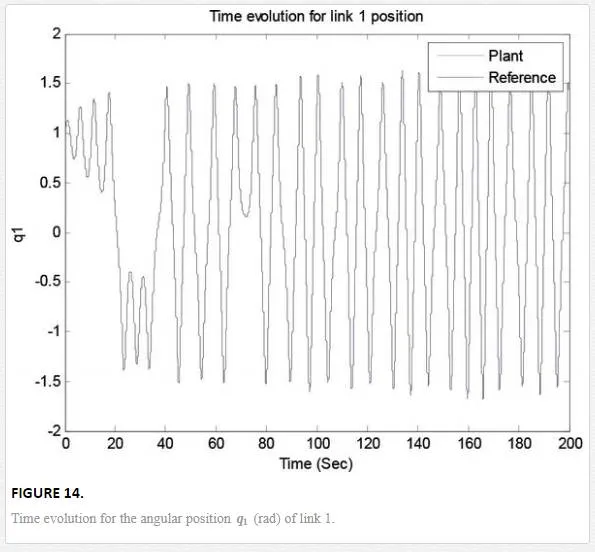
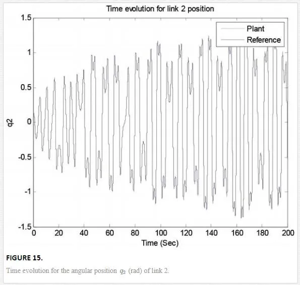
Its phase space trajectory is given in Figure 13, and the time evolution for the position angles and applied torque are shown in Figures 14–17. As can be seen in Figures 14 and 15, the trajectory tracking is successfully obtained where plant and reference signals are the same.
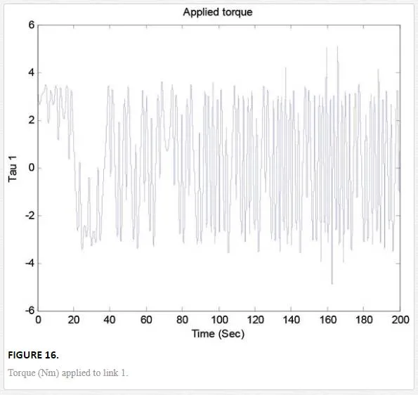
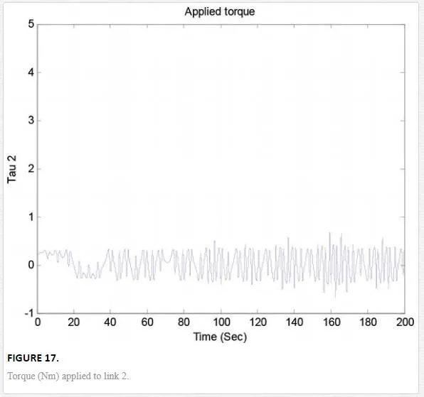

As can be observed, in the graphs of the trajectory tracking, the experimental results obtained in this chapter show a good experimental performance. The laws of control are obtained online, as well as the laws of adaptive weights in the fractional order neural network.The control laws obtained are robust to modeling errors and nonmodeled dynamics (unknown nonlinear systems).
Conclusions
We have discussed the application of the stability analysis by Lyapunov of fractional order to follow trajectories of nonlinear systems whose mathematical model is unknown. The convergence of the tracking error is established by means of a Lyapunov function, as well as a control law based on Lyapunov and laws of adaptive weights of fractional order dynamical neural networks.The results show a satisfactory performance of the fractional order dynamical neural network with online learning.