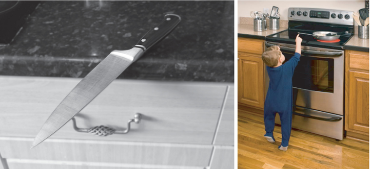
The concept of automated risk analysis for domestic scenes is a developing area of research, where the goal is to allow the quantification of measurable elements of risk into some sort of coherent risk score. With the definition of a risk score, thresholds can be defined to trigger certain actions, this might be a cue for a robot to find an alternative route through an environment or to take action to reduce the discovered risk. Humans and robots are almost constantly exposed to risks in one form or another. As humans, risks are identified and appropriate actions are taken almost on a subconscious level and as a result we are excellent at self preservation. To date robots have lacked these mechanisms despite an equal need to ensure their own protection.By providing the functionality to detect these potential risks, advantages are gained in two ways, firstly the robots themselves are given an awareness of potentially dangerous scenarios and therefore become better able to protect themselves from damage. Secondly, the risk detection abilities can be utilised for those at risk members of society whose hazard perception capabilities are diminished or underdeveloped.
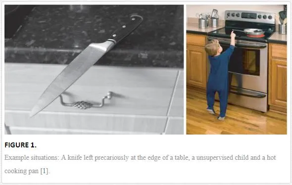
As an example, most people will make use of a kitchen in their daily routine and the act of leaving a knife near the edge of the sideboard would not pose a significant risk (Figure 1). Consider now the same scenario but with an elderly adult suffering from Parkinson’s disease or early onset dementia being the user of the kitchen, or with a child running around the room. The possibility of knocking that knife on the floor for a healthy adult is low, but for a child not actively aware of their surroundings or those suffering from a disability this could become more of a likelihood, likewise without suitable software governing interactions, a robot could equally suffer from the results of a falling blade.
Invariably there is a percentage of society that could be classed as more at risk than the rest. For example there are an estimated 10 million disabled people living in the UK [2] and the elderly (65+ years) and young children (<10<10 years) account for 28%28% of the UK population [3]. People within this age range are statistically more likely to have an accident in the home [4]. Additionally the number of people that fall into the elderly category is increasing. Europe has one of largest ageing populations with 24%24% already aged 6060 years or over, this is set to increase sharply such that by 2050 that proportion is projected to reach 34%34% [5]. As such the infrastructure which provides continued support services to this population will come under increasing pressure. With this increase in the amount of elderly adults continuing to live self sufficiently, the need to alleviate the stresses on the support services and the need to provide a high level of care, emerging technologies can be used to ensure they remain safe and if something were to happen, appropriate services can be notified or actions taken.
The International Federation of Robotics (IFR) have noted a steady increase in the sales of professional and personal robotics since 2012, with predictions that during the period of 2014–2107 the estimated number of service robots sold for domestic/personal use could be as high as 27 million [6]. With this emergence of more and more domestic robotics, these devices also face similar risks and require similar systems by which to identify risk. This may be within the bounds of keeping an at risk user safe, for example a domestic robot ensuring that a room is safe for a child, or just keeping the robotic system itself operational by ensuring the path it intends to take is free from potential hazards [7].
As such automated risk assessment research provides the facility to measure risk, resulting in a numerical scaling upon which thresholds of risk can be defined and appropriate actions taken. The increase in the availability of these technologies and the integrated vision hardware that is often incorporated, provides the ability to analyse hazards for those at risk individuals within a domestic environment. The primary form of computing these risk scores is through the use of a risk estimation framework which provides a basis from which a combination of measurable elements of risk can be output into a risk score for a given environment. Existing approaches to the definition and measurement of hazards include the detection of risk related objects [8, 9] scene stability [10, 11] and human behaviour simulation [12, 13].One of the primary issues when looking at a unified approach to risk estimation is the problem of context. In short the importance of ensuring that a provided risk score is relevant to the end user regardless of situation. This is due to the fact that what can be considered safe in one environment may not be in others. For example, a container of liquid at the edge of a table is risky in a household environment however in a chemical laboratory this might pose a far larger danger.
In this case stability estimation would need to take precedent over the prevalence of hazard features or behaviour analysis. Similarly users of the environment will also affect how risk is perceived; if the environment contains children or elderly adults the threshold of what is considered risky may need to change. However, regardless of context, the elements that might contribute to the concept of risk can be broken down into components from which a decision can be made. These components include elements such as shape, size, material, temperature, position as well as many others.An area of risk evaluation that has yet to be fully explored is the effect interaction with an environment has on a potential risk. Take again the example of a knife balanced at the edge of a table, alone this poses no hazard, however if there is a likelihood that there will be some interaction with the knife then the scenario develops into something more hazardous. Additionally the human response to risk opens up potential new threats as the behaviour of an agent in a scene will differ based on the presence of hazards. As such the ability to define these interactions and, on an environment basis, predict them allows for a more accurate assessment of risk in a scene.
To this end the focus of this chapter is the introduction of automated risk analysis research methods that can be used in scene analysis tasks to measure risk. As such the forthcoming sections will continue as follows; Firstly an overview of the base risk estimation framework [14] with a brief analysis of some existing risk elements. Next a focus is given to the concepts of risk analysis relating to interaction through the use of behaviour simulation. As such simulation techniques relating to risk are introduced which can be utilised as prediction mechanisms, evaluating likely interactions between environment and user. Finally simulation evaluation is discussed, ensuring that suitable and appropriate validation techniques are used to verify the simulation outputs.
Research methods
Within the following sections a overview of existing risk estimation techniques will be given. Starting with a base framework from which different measurable elements of risk can be combined to give a robust and relevant evaluation of a scene’s risk.
THE RISK ESTIMATION FRAMEWORK
The risk estimation framework as defined in Ref. [14], outputs a risk score from measurable elements of risk. As such the cumulative risk score, RR, for a scene is defined as the weighted sum of nn measured risk elements ee (Eq. (1)). The weighting specified for each element should fall into a range from zero to one, with the sum of the weightings for all included elements being equal to one.

The use of this weighting of elements allows the consideration of the aforementioned issues regarding the context in which the risk is found. Allowing the final system to tailor its outputs, applying more weighting to elements that are more relevant in a given situation.
RISK ELEMENTS
A risk element represents any scene property that may present a danger and is given as a quantitative measure that could highlight those potential risks. An obvious example would be temperature obtained from a thermal camera. To date existing work is risk estimation has provided techniques, and thereby risk elements, for the detection of risk related objects [8, 9] and scene stability [10, 11]. With this concept of risk elements and an established, flexible framework, the concept of defining risk in terms of environment interaction and behaviour analysis allows for smart enabled homes or domestic robots to analyse an unknown setting and build up a detailed map of the potential risk.
RISK RELATED BEHAVIOUR SIMULATION
In June 18831883, the magazine The Chautauquan, posed the question, ‘If a tree were to fall on an island where there were no human beings would there be any sound?’. The proposed answer was no, given that sound is a human’s perception of movement in airwaves. If there is no one there to perceive those movements then there cannot be any sound. This concept is loosely the basis for risk analysis based on interaction. If there is a boiling beaker of acid, perched precariously close to the edge of a table, but no‐one ever goes near it. Is it still a risk? In reality, yes, but far less so that if that table was situated in the middle of a busy train station at rush hour. As such a method is needed by which the prediction and analysis of these interactions can be used to contribute to the risk scores detected within a scene.
ENVIRONMENTAL RISK MAPS
To simulate interaction with an environment it is important to consider a number of aspects. Firstly and most notability, the expected paths that humans or robots would take through a scene (Figure 2). Second to this is the concept of visibility, how much of the scene is visible to the average human as they navigate the environment. For example if a path passes near a table, the top of that table is likely visible but below or behind would not be. Additionally the concept of redirection on account of a hazard must also be taken into consideration, allowing for the fact that paths though an environment may change on account of a discovered risk. As a result of this redirect, other areas within the environment would have an increased likelihood of interaction.
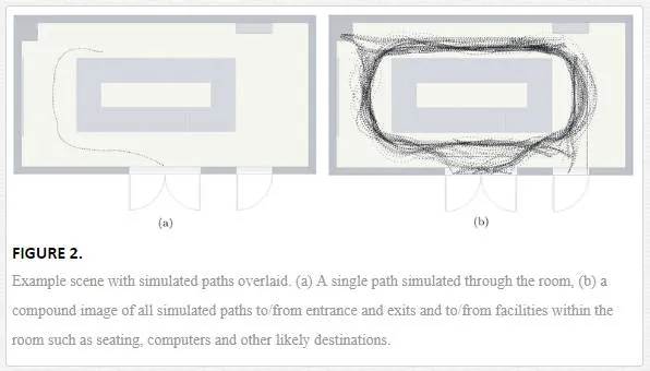
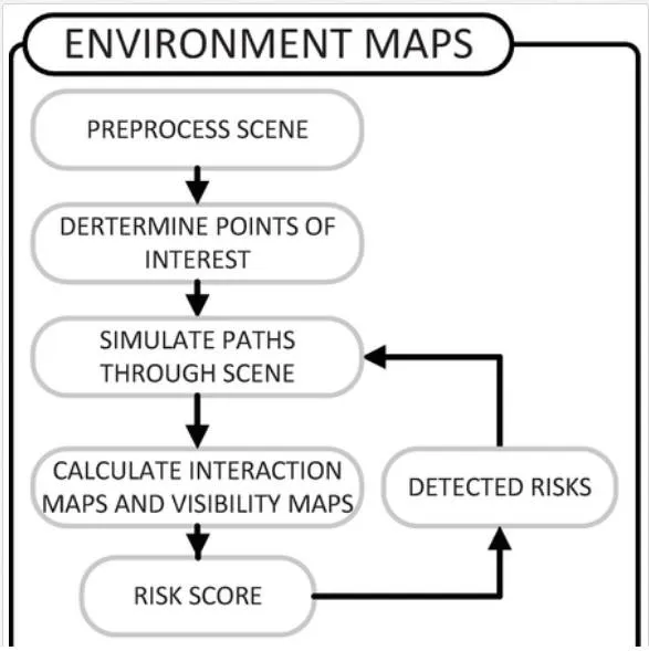
Figure 3 outlines this process. Initially a scene is preprocessed to obtain a 2D mapping or floor plan, interest points are then extracted and paths through the scene are simulated. The environmental risk map is then calculated, providing localised risk scores for the whole scene. Finally, simulations can be re‐run based on the presence of risks detected by any other part of the risk estimation framework
INTERACTION AND VISIBILITY MAPS
By tracking a human or robot’s movement through an environment over time a map can be created describing which areas are used more frequently than others. However method requires long term observation and is specific to each individual environment. As such utilisation of behaviour simulation techniques allows for similar results in a fraction of the time.Initially to allow simulation of an environment to be run, mapping of that environment is required. This can be achieved through a number of methods [15–18] with the detection of entrances through use of existing techniques [19]. By creating a low resolution two dimensional map of an environment, with labels defining points of interest, multiple simulations can be run to replace the long term monitoring techniques.
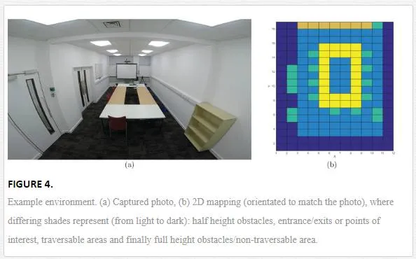
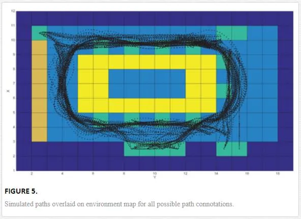
Using a two dimensional Cartesian representation of an environment a movement space in terms of xxand yy coordinates is defined. The mapping represents a low resolution view of the environment, where one unit square maps to a set square measurement in the environment (e.g. 0.5m0.5m). Obstacles in the environment are also represented in the map, allowing the agents in the simulation an awareness of what is traversable and what is not. An agent in a simulation can be used to represent anyone or anything that can interact with the environment, in our case it could be a at risk adult/child or a domestic robot. Figure 4a shows an example environment in which a meeting room is shown with a set of tables arranged in the middle of the room, Figure 4b shows the 2D environment map of the same scene.Using the defined entrance/exit locations and points of interest, an exhaustive set of paths that take into account all possible path connotations can be made. For each one of these paths a simulation is run in which an individual agent, representing a human or robotic subject, traverses the environment from a start location to a destination, avoiding any obstacles that may be in their way
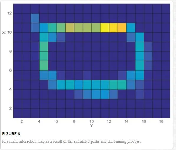
The results of an individual simulation provides positions P=[x,y]t∈R2P=[x,y]t∈R2 for an agent at a specific time tt. By removing the time component and plotting these points in the movement space we build up a picture of a single traversed path, similarly plotting all the paths from all the agents demonstrates areas that are most commonly used (Figure 5). 2D histograms are then created by binning each individual position, of each agent, at each time, into its respective unit measure within the environment map (Eq. (2)).

where ii and jj represent bins or unit measures within the scene along the xx and yy axis respectively of the environment map. The sum of points within each bin is used as a measure of frequency, (Eq. (3)). The result is a low resolution frequency map, indicating areas of high and low interaction (Figure 6)
| Hi,j=∑k=1thi,j(Pk)Hi,j=∑k=1thi,j(Pk) | (3) |
Thus locations of high frequency define areas in the environment in which the simulation algorithm estimates a higher level of human presence, as such these areas would present more of a risk than those of low frequency.Using the same simulation techniques and histogram principle as Eqs. (2) and (3), the concept is expanded to encompass the visibility component of simulated agents in an environment. Each agent within the simulation has a number of defined properties, these include agent radius, movement speed, acceleration and turning speed. In addition to these a number of properties are defined that pertain to that agent’s ability to see the environment. A field of view is defined as F=[ϕ,q]∈R2F=[ϕ,q]∈R2 subject to νν, which specifies the angular range of that agents peripheral vision ϕϕ, as well as a viewable radius qq
where νν is a value from zero to one defining how well an agent can see at a specific point of their vision. In the case where the agent is representing a human, closer and more central points are better seen and those at the edge of an agent’s vision and further away rated worse. This can be based on a logarithmic scale [20] for humans, however a more comprehensive model of visual acuity in human peripheral vision could be applied. Likewise for robotic vision, visual acuity would also be defined depending on the sensing devices equipped to the device. For example, the concept of diminishing acuity at the edge of perception may not be applicable. During the simulation an agent’s viewable area is recorded per time instance, subject to an agent’s properties. Within the context of the environment mapping this is defined as whether an agent can see a specific unit square of the map or not (Figure 7)
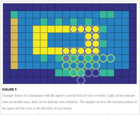
Parameters for field of view and peripheral visual acuity allows the tailoring of the environmental risk maps to better reflect those that use the environment. As in the cases of children, the visually impaired, or the elderly who have reduced peripheral visual acuity or Tunnel Vision due to conditions such as glaucoma or brain damage the risk of visibility maybe a more important factor, likewise for robots vision maybe less of a consideration than just the interaction component.The 2D map of the scene is updated to reflect the differing heights of obstacles, such that a label is defined for obstacles that can be seen over and for obstacles that cannot (Figure 4b). For example, walls fully obscure the agents view, however low height obstacles, such as tables, block vision directly behind them but allow vision further away. As can be seen in Figure 7, where the area in the centre of the room cannot be seen as it is occluded by the presence of the tables, where as the table across is still visible to the agent.As before simulations are run for the given connotations of paths. Position is extended such that P=[x,y,ν]t∈R3P=[x,y,ν]t∈ℝ3 where νν represents how well that position was seen by the agent at that time subject to (Eq. (4)), as they navigate through the scene on their estimated path (Figure 7). The 2D histogram continues to bin based on location, however the contribution to the bin is now made by the visibility component (Eq. (5)).
The visibility map is then given as the summation of the histogram bins over time as (Eq. (3)).
Figure 8a gives an example of a single agent’s track with the compounded visibility map for that path shown in Figure 8b. The same method is used for all the given path combinations and a single compound visibility map returned for that environment (Figure 9).
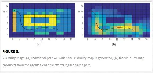
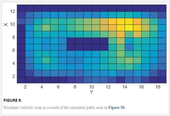
The higher the visibility values recorded for an individual unit square of the environment map, the more often and better seen that area of the environment is likely to be. Conversely those areas with low values are not well observed and could further add to a hazard at that location due to its potential to go unseen. As visibility is a positive measure and the risk scores to date are negative measures, the visibility histogram needs normalisation and inverting (Eq. (6)). As a result the histogram, HVHV, then provides a measure of invisibility, within a range of zero to one.
The final risk element EE for the environmental risk maps is given as a combination of the risk associated with the presence of a person or robot and their ability to see hazards in a given environment. As such a weighted combination of the histograms produced by the interaction maps HIHI and the visibility maps HVHV is given as
where ww represents the histograms contribution to the final risk element and the two contributions wV+wI=1wV+wI=1. The weighting is flexible based on the final implementation allowing the condition of those using the environment to be considered during simulation.
SIMULATION
To generate the position data used in the environmental risk maps, simulation algorithms are used to replicate the behaviours of those that interact with the scene. Simulating behaviour is often considered to have started with Reynolds work in 19871987 with the emulation of animal behaviours [21]. Within Reynolds’ work the concept of steering simulation was introduced, whereby each individual agent in a scene has its movement governed by a set of rules. In this case each agent follows three rules: steer towards the goal, steer away from the nearest obstacle, and steer away from the nearest person. Later Helbing et al. [22] introduced the Social Force Model (SFM) which uses potential fields defined by neighbouring agents to impart an acceleration to each agent. SFM’s compute the trajectory of each agent by applying a series of forces to each agent that depend on the relative positions and velocities of nearby agents and the goal of the agent (Eq. (8)).
where gaga is the current destination of the agent aa to its final goal, with papa being the agent’s current position. The forces for separation, f(a,bi)f(a,bi), object avoidance f(oj)f(oj) and predicative agent avoidance f(a,bk)f(a,bk), is calculated for any relevant entity within a defined neighbourhood.
The simulation techniques described above relate to the local movement of agent from frame to frame. The overall path the agent follows through a scene is extrapolated at a higher level. Given a pre defined destination an agent performs a route plan using the A* algorithm to estimate the most direct course through the environment. A* is often used as it provides a near optimum path through the environment whilst being computationally efficient enough that it can be run on demand in real time if required [23]. Given that the intended applications for this work are likely indoor environments and may well be computed within the confines of a domestic robot, considerations as to the speed of runtime and algorithm applicability are important.These simulation techniques govern local movement but not the overall strategy of the agents. With the integration of these factors, more rounded behaviour simulations began to be developed. The integration of risk related concepts into simulation algorithms has been a recent development, allowing for the prediction of crowd dynamics and behaviour in the presence of a stressor. This is especially important in areas such as architecture and engineering where through simulation more efficient evacuation plans and facilities can be built.Kim et al. [24] focus on the modelling of the human perception of risk and how that subsequently effects behaviour. Using the general adaptation syndrome (GAS) model, proposed by Hans Selye (1956) [39], which acts as a model for the general response to any stressor (toxins, cold, injury, fatigue, fear, etc). The GAS model has three stages of response (Figure 10): alarm, the agent perceives a stressor and readies themselves for the ‘fight’ or ‘flight’ response. Resistance stage, in which agents work to resolve the stress at their full capacity and finally if the stressor is not resolved, they reach the exhaustion stage and resistance becomes futile.
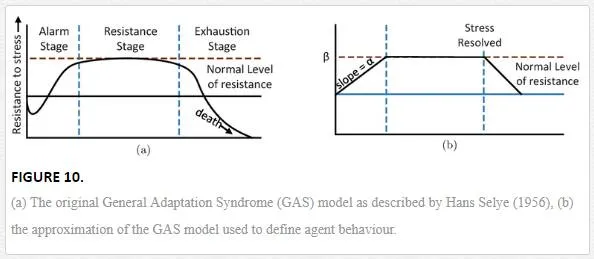
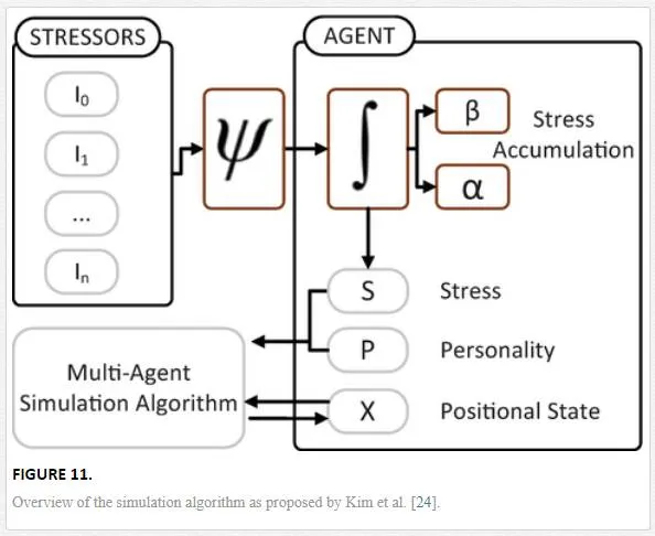
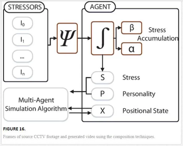
Within this work, the goal is to approximate this model and apply the results of the various stages to the agents in a scene. This could range from mild stimulants, such as challenging situations (e.g. time constrained events) to threatening situations such as fire. These stressors are split into a number of categories from positional stressors, e.g. the effect on an agent from being in a certain risk area or the increasing effect of a stressor based on its proximity. Also the concept of interpersonal stressors is modelled, which allows the agent to perceive stress based on those around, for example crowding. Figure 11 highlights the overview of this process, where I1…nI1…n are the stressors. PP represents an agents stable personality, which, given no stressors, would define the variables to drive the simulation algorithm. ΨΨ is the perceived stressor function. ββ and αα control the agents stress response SS, this defines how an agents responses will be effected in the presence of a stressors and is based on real world data. This directly impacts the way in which the agents act both at a personal and global level. Changing the way they react to others in the scene as well as driving decision making abilities regarding where they are going. Finally XX represents the positional data of each agent and the resultant output of each frame of computation.
The addition of this stressor consideration allows for agents in a scenario to disregard common psychological behaviour effects that maintain coherent movement such as separation from those around. Instead the agent focuses on reaching their perceived goal as fast as possible. Through this addition the ability to model instances such as building evacuations under stress become more accurate. As a test case, the scenario of the Shibuya Crossing in Tokyo is utilised. In which agents are exposed to a mild time constrained event in which they must cross the road in the presence of many other agents and within a limited period. A quantitative assessment is made by looking at psychological study of pedestrians crossing roads [25], comparison is made of variables such as average crossing speeds against how much an agent has been delayed entering a street crossing from the start of the signal. This is then compared with the outputs of the simulation to provide a similarity measure.
Furthering this concept of modelling the perception of risk and how it effects behaviour, Klugl et al. [13] creates a model that aims to simulate an agents response to the evacuation of a train with an engine on fire in a tunnel. In this case rather than the perception of risk effecting their local movement, it is the decision making capabilities that are focused on. This is due to the need to understand what a agent would do in a given situation and allow the development of evacuation plans that compliment this. As such the cognitive model focuses on the perception of the risk, in this case fire, by the agents exposure to smoke and increasing temperature as well as other agents ‘knowledge’ of where the fire is located. Additionally factors such as visible signage and congestion, all effect the agent’s strategic thinking for exiting the train tunnel. Exits are given as either the end of the tunnel or specific emergency exits. Figure 12 demonstrates how the decision making components of the model effects the local movement, as well as an overview of how the decision making process is made.
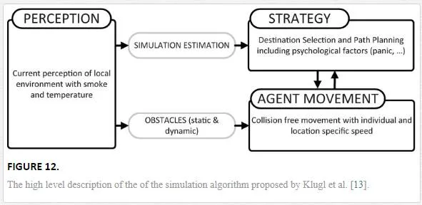
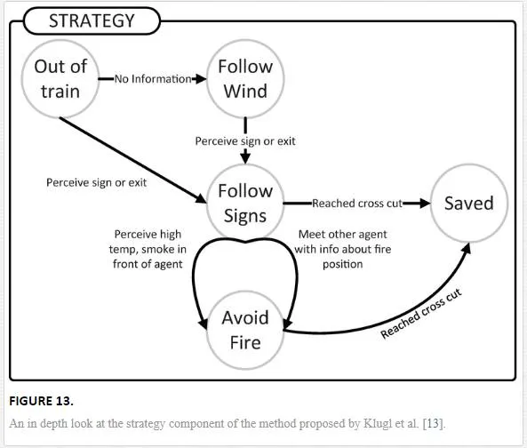
A number of variables in the agent movement model are dedicated to the representation of risk to the agent. Panic variables are used to increase movement speed and reduce the agents concept of personal space. Although this is a less complex representation of the agents perception of risk, Klugl does provide a more in depth look at the conative decision making processes which allow for an agent to adjust their goals given the presence of a hazard and utilising available new information (Figure 13).
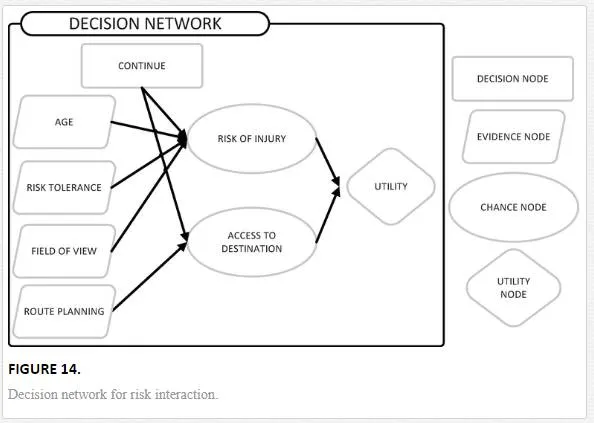
Using this focus on the higher level decision making process, utility and probability theory [26] can also be applied to the problem. Given that in a domestic environment the hazard situations that are encountered are likely to be less severe, the effect of panic on an agent is less of a priority. Instead focus should be on the reaction to the risk and whether that changes the way an agent interacts with environment. For example if a parent discovers a broken glass on the floor they will likely ensure that any children present will navigate through an environment differently or avoid it all together.Therefore by applying utility theory, predictions on how interactions change in the presence of risk can be made. In any given situation, the action an agent will take is defined by a set of probabilities. In the domestic situation the agent decides to either continue on their existing path or recalculate a new one to avoid a risk. As path finding and an agent’s local movement are governed by other aspects of the simulation algorithm it is only this risk related choice that requires a decision making process.
Let SS be a state at a given time in a simulation for an agent. Figure 14 outlines this decision process for state SS as a decision network. Within the diagram the decision node represents the problem to be resolved by a set of actions AA. In this case which action to take whilst traversing the environment (continue or reroute). The chance nodes are indicative of the probabilistic outcomes associated with this decision represented as probability distribution functions. In this case the chance of injury and the chance of being able to find a path to the destination. The evidence nodes represent the knowledge the agent has, which directly affects the chance nodes. For example the risk of injury will change based on an agent seeing a hazard. Finally the utility node is the utility or value for the state SS based on the chance nodes and an agent’s preference.
To determine the best action for the agent to take, the principle of maximum expected utility (MEU) is utilised in 9. Here the possible actions AA are assessed using the expected utility EUEU, based on the known evidence EE. Therefore the MEU represents the action AiAi which is classified as most favourable by the agent.
Evidence is a combination of agent variables and environmental feedback, for example for a human E=[pa,pr,pp,pf]E=[pa,pr,pp,pf] where papa is the age of the agent, prpr is their tolerance of risk (represented by Gaussian distributions, assuming prior knowledge of the means and standard deviations of the relevant information), pppp is the presence of an alternative route and pfpf represents a seen hazard. In this simulation environment there are two actions that can be taken by an agent representing a single decision; continue on their preplanned path, or reroute to avoid the hazard.
The expected utility of an action is defined in 10. Expected utility represents a measure of both the likelihood of a particular state occurring, combined with the agent’s preference for that outcome. Here a possible action AA has a number of possible outcome states Resulti(A)Resulti(A). For each outcome a probability is assigned based on the evidence EE. Do(A)Do(A) represents the supposition that the action AA is executed in the current state.
The given probability of each action AA is then multiplied by a utility function UU for the possible outcome states. In this example the utility function is simplistic as only a limited number of states exist based on the decision network presented in Figure 14. The utility associated with accessing the destination will nearly always take precedence; if the direct route to the destination is accessible then the agent will continue, only in cases where risk of injury is high will the agent decide to reroute. However if the route is blocked then regardless of the risk of injury the agent will have to reroute.
As an example, in a normal situation with the absence of risk, the probability associated with risk of injury is low and the probability for reaching the destination is high. Given that the agent wants to get to the destination, whilst avoiding injury, the EU(A|E)EU(A|E) for the AA to carry on the current path is high. However if the evidence changes and a risk is detected through an agent’s field of view, the probability of risk of injury increases. If there exists an additional route the agent can take to avoid the risk, the EU(A|E)EU(A|E) for the AA to reroute will be higher and therefore the preferred option.
As a result of these simulation techniques a detailed representation of environment interaction can be created and used as the bases from which the environmental risk maps can be computed. However as with any simulation algorithm the evaluation of how realistic it is a complex problem, defining how realistic the simulation outputs are impacts the accuracy of the interactions maps, and therefore the accuracy of the produced risk evaluation. As such the topic of simulation evaluation is reviewed, providing a number of examples of how the validation of the simulation methods can be done.
SIMULATION EVALUATION
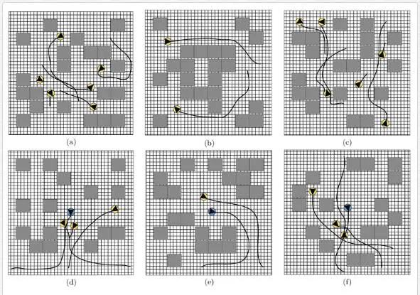
One of the most prominent issues with behaviour simulation research is the lack of a simple and suitable form of evaluation from source data to simulation output. This task is made more difficult as the developed simulation approaches cover a huge range of applications, where evaluation techniques for one are not always applicable to the others. Generally the evaluation techniques utilised can be split into qualitative [27] and quantitative measures [24, 28]. The former including assessments made by experts in the field or context of the intended application [13], as well as category based rating systems [29] designed to define the capabilities of an algorithm (such as emergent behaviours).The ability to have a single value or set of values to define how good a simulation is, is a favourable goal and requires analysis of the outputs of the simulation algorithm. Kapadia et al. [30] look into the assessment of simulation algorithms using an exhaustive test case format. Evaluation of a algorithm is based on its ability to navigate ‘steering problems’, i.e. the traversal of a scene to a predefined goal, whilst avoiding both static and dynamic objects. Using procedurally generated steering problems, a specific simulation algorithm can be tested across a broad range of scenarios. To facilitate this, two notions are presented: the first is the concept of scenario spaces, and secondly, metrics to quantify the coverage and the quality of a simulation algorithm in this space. Scenario space is defined as a set of parameters from which environments can be generated to test a simulation algorithm in. These values consist of upper and lower values for numbers of agents, obstacles and environment size amongst others. Figure 15 demonstrates some example steering problems taken from a scenario space. A successful generated space must adhere to a set of rules, for example an agent must be able to get from its origin to its goal and, on initialisation, there should be no collisions between agents or objects. A successfully completed scenario is defined as a boolean value, completed or not. To meet this a simulation algorithm must navigate an agent through the environment within a fixed time and without colliding with other agents or static objects. This process is repeated for a representative number of possible combinations derived from the scenario space.Evaluation of the successful spaces is done based on three metrics: scenario completion, length of time and distance travelled. These are compared to optimal values calculated when generating that specific test space. Using these metrics, concepts of coverage, quality and failure are computed for a given simulation algorithm for a given scenario space. By substituting different algorithms and using the same scenario spaces, comparisons between algorithm performance can be established.
This exhaustive form of analysis is useful in testing the limits of a given simulation algorithm and highlighting types of scenario where a particular method might be improved. In addition the automated nature of the test generation provides a useful platform from which easy benchmarking can be performed. However, the exhaustive randomly generated scenario spaces that are created lack similarity to real world scenarios nor is any real comparison made with source data.As such the next logical approach is the development of a comparative system which can use source data as a comparison or benchmark from which to evaluate the output of simulation algorithms. This could provide overall similarity ratings but also more localised analysis, whereby areas of interest or high deafferentation could be highlighted specifically. Alternatively the simulation outputs themselves can be analysed for outliers, highlighting possible anomalous data relative to the rest of the outputs.
One such example is the work of Charalambous et al. [31] in which a data driven approach is applied to the problem by developing an analytics framework for anomaly detection. Unusual behaviour is principally presented using two processes. Firstly outlier detection which takes a set of data and analyses it with no other reference data, allowing for the definition of odd behaviour within just that dataset. Secondly novelty detection, in which sample data is compared to reference material to find and describe trends or actions that differ from the reference data. Using segment analysis of agent trajectories, a set of metrics are used to characterise each portion of the agent track, these include properties such as average speed, maximum curvature or minimum distance to nearest neighbour. Using this set of metrics, a nominal data representation is created for that dataset, this can be used as training for similar unseen data. Which metrics are used to create this representation of nominal data is user defined and will vary based on the types of data and the scenario. Using techniques such as Once Class SVM, Localised p‐value estimation (kk‐LPE) and kk‐NN Based Approaches, outliers in the test data can be highlighted. Off the back of this analysis a set of user‐in‐the‐loop analysis tools are created, which provide an interface by which to interpret the data. Due to the low level analysis of the simulation this can localise specific agents that are acting erroneously or where general areas of inconsistency appear in the test scenes. Another alternative to data driven evaluation approaches is through the use of visual comparative frameworks. This builds on the notion that a simulation’s accuracy is not entirely based on its ability to reproduce specific agents movement exactly, rather the concept of similar looking simulations are considered better. This provides a more general approach to evaluation and replicated better the natural formation of crowds. For example people moving through a train station day to day will follow similar paths, but will experience very slightly different crowd dynamics, likely causing them to vary their path slightly from the previous day. This would represent a change in behaviour but not necessarily an anomalous one. Regimented data driven techniques do not allow for this variation and ignore whether the crowd movement looks similar.
The following framework makes use of compositing techniques and video analysis tools to compare source footage to simulated. Evaluation can be done on a frame by frame basis or on a sequence as a whole, providing flexibility in how the simulation is evaluated. Additionally the methodology requires no track or path information from the source material, allowing any video footage captured from a static viewpoint to be used.Comparison is made using the original source footage and a video created using composition techniques, in which simulated agents are superimposed into the background of the source video data (Figure 16). A set of metrics designed to evaluate the visual similarity of the two videos is used to provide a quantifiable similarity metric. These are designed to emulate the way the human visual system (HVS) perceives motion, both in direction and volume. Fundamentally the framework is made up of two components; simulation visualisation and video similarity.
Figure 17 provides a brief overview of the process. As the framework compares video data to derive a similarity value, firstly a simulated video must be constructed. Using the source video sequence, the background is extracted. A two dimensional plane representing a top down view of the given scene is used as the simulation space. Simulations are run to produce paths for virtual agents to follow based on the extracted plane. The visualisation component is used to composite the extracted 2D background image and 3D rendered agents as they follow the simulated paths. Frames are output from the visualisation into a final simulated video sequence (Figure 16). Once both a simulated and source video are available, the similarity can be evaluated. Optical flow and tracklet analysis are run and features extracted from the subsequent data. Finally a distance measure is used to analyse the difference in features to give the final similarity metric.
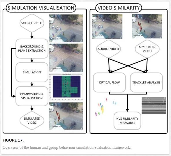
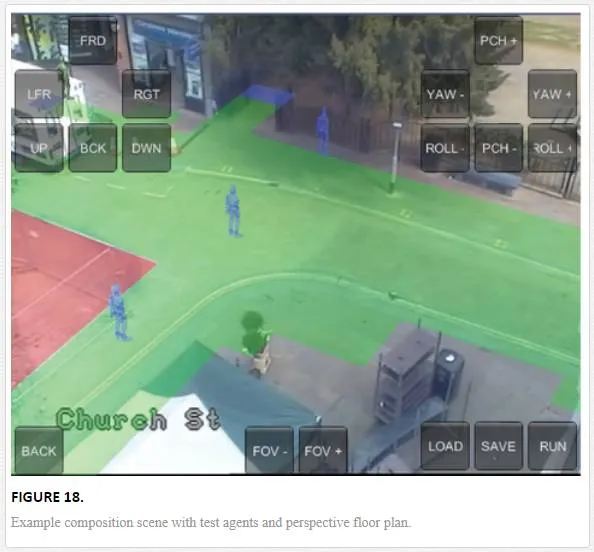
The visualisation stage of the framework performs the composition of a scene. Firstly the background of the source video is extracted using gaussian mixture models [32]. Next a perspective plane is generated in 3D based on a 2D mapping of the scene, this could be obtained during the environmental maps evaluation. The key to a visually similar composition is the positioning of a virtual camera at the same location as in the original scene, relative to the perspective plane. By using layers the camera can have the source image as a background and visualised 3D agents, controlled by the simulation, superimposed. When correctly aligned the illusion of the 3D agents walking through the scene is created. This alignment can be performed manually using the position and orientation of the camera or automatically using camera calibration techniques [33, 34]. The 3D agents in the scene must also be scaled correctly to ensure their sizing is appropriate to the scene (Figure 18), this can be done manually or calculated automatically using the methods provided in Ref. [35].
To produce the simulated video, the 3D agents navigate through the scene with the virtual camera capturing composite images. For each frame of the visualisation the agent location and rotation is updated based on the simulation algorithm output. Once visualisation is completed the individual frames are compiled into a video sequence.
Once the composite video sequence is complete, the source and the simulated video sequences are used to extract human visual system’s (HVS) features in order to measure their level of similarity. These features are based on the optical flow [36], Histogram of Oriented Optical Flow (HOOF) [37] and tracklets [38] of the moving objects in both sequences and are designed to emulate the way in which humans perceive motion. The feature representations used highlight different properties of video sequences allowing for a specific analysis of a simulations output, for example tracklet analysis allows for the pathfinding component to be evaluated, similarly the histogram of optical flow provides a good analysis of crowd volume and speed.In order to evaluate the similarity level of the simulated and source videos using the HVS features, a metric is required that will allow an objective comparison of the extracted features. The Bhattacharyya distance measure is utilised, providing an individual score of similarity between each video sequence across the features used. This can be expanded to a frame by frame, or even a block by block analysis, allowing spatio‐temporal adaptation of the metrics. With this utility the final distance metric can highlight area of the video sequence which seem dissimilar from the source. Additionally through the comparison of individual features the type of analogy can be deduced.
Conclusion
The task of automated risk assessment in a domestic environment is an emerging area of research. The issues surrounding the identification, classification and, finally, quantification of risk are substantial. There are the practical issues of identifying a risk or hazard, as well as the contextual problem of defining what is considered as hazardous and what is not, both of which are non‐trivial tasks. One such issue is the effect that human interaction has on detected risks in an environment and conversely the effect those risks have on those within the environment. More importantly methods are required to predict these effects and therefore provide further insight into those detected risks, allowing for a more complete picture of risk in an environment.
An introduction to risk as a function of interaction has been given in the form of environmental risk maps, which quantify presence and visibility to provide an risk element for use in the risk estimation framework. Environmental risk maps rely on the accuracy of the simulation algorithm used to produce realistic behaviour in an environment. This forms the basis from which the interaction and visibility components of the environmental risk maps are calculated, ensuring that outputted risk scores are logical and relevant.As has been demonstrated the definition of simulation algorithms and models for predicting behaviour is a challenge, primarily due to the need for careful consideration when defining which aspects of human or robotic behaviour to model. This issue is exacerbated when modelling behaviour in the presence of risk. Crucially this simulation data is utilised for the definition of environmental risk maps, and therefore the accuracy of the simulation must be verified to ensure that the produced behaviour and by extension the produced risk scores are realistic. There is ongoing development in this field for the parametric definition of behaviour, i.e. which elements of behaviour effect the way we navigate and move? Extension of these parameters would allow for a more tailored approach to the simulation of agents in a scene, allowing more specific emulation of robotic devices or humans with disabilities or limitations, however this requires a detailed analysis of which factors need to be considered and how applicable they are.
A number of simulation techniques have been reviewed looking at the various aspects of behaviour modelling from movement mechanics up to the strategic decision making functionally. Finally as validation of simulation accuracy is vital to the relevance of the environmental risk maps a number of simulation algorithm evaluation techniques have been reviewed. A broad introduction to the topic has been provided in the form of exhaustive procedural analysis techniques through to outlier detection and data driven comparisons, finally a novel composition based analysis framework emulating a human’s ability to identify similarities in movement is also reviewed.Domestic robotics and smart homes are a growing industry and will become an integral part of life in the near future. Currently available commercial products aim to perform menial tasks, simplifying processes that humans perform every day. For example taking notes, the initialisation of domestic appliances, information retrieval and simple household chores. However with the ever more interconnected nature of the domestic environment and the availability of increasing computational power, these devices will take on new roles. The ability to provide basic decision making capabilities as well as more detailed interaction and analytical abilities will enable the application of more complex behaviours in these devices.
In a domestic setting this will likely lead to the performing of more complex tasks such as assisting with a wider range of household chores, heavy lifting and entertainment. However for scenarios involving the presence or potentially the monitoring of those that use the environment (e.g. children or at risk adults), elements of risk detection will be required to ensure user as well as device safety. These concepts will be required in the emulation of further higher level behaviours and will produce an initial step in the development of systems that can make a real difference in easing some of the impending social issues to do with health care and ageing populations. However with these developments also comes a vital need for the establishment of independent advisory and certification boards. These organisations would provide governance on the usability and appropriate audience of the various devices and in doing so provide minimum safety requirements for use with humans as well as practical guidelines for device preservation.
