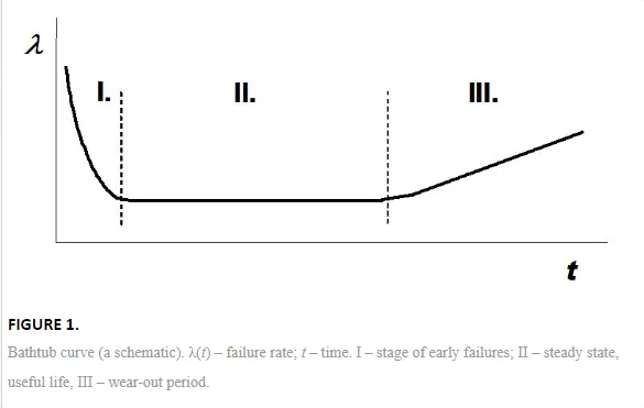
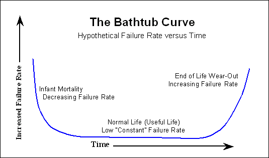
Failure rate, can change with time. Figure 1 shows the time course of λ(t) typical of nonrepairable objects, such as electrical bulbs, pumps, switches, or springs, and also living beings, including humans. Such course can be obtained if the operation of a high number of objects of the same kind is monitored. Due to its shape, resembling a longitudinal section of a bathtub, the curve has got the nickname bathtub curve. It can be divided into three stages with characteristic time courses related to different reasons of failures.

Stage I. Failure rate λ(t) is high at the beginning and decreases with time. The failures occur due to errors in design, weak components or inferior materials, due to faults appearing during manufacture or building, or due to mistakes caused by an inexperienced personnel or user. A weak newborn baby more easily succumbs to an infectious disease. Software errors also belong to this category. The failed components are discarded and not used any more, the customer gradually becomes familiar with the use of a product, and the errors in software are corrected. This period is called the stage of early failures or infant mortality.

Stage II. Failure rate λ is low and approximately constant. In contrast to early failures, caused by the inherent weakness of the object, the failures during stage II occur mostly due to external reasons, such as overloading, collision with another object, weather or natural catastrophes, hidden defects, and mistakes of the personnel. (In the case of people, the reasons for the “failures” during this stage are traffic accidents, diseases, wars, and murders.) Depending on the object and conditions, failure rates for various objects can be very different. Stage II represents the major part of the life and is called the useful life or the period of steady-state operation.

Stage III. Failure rate λ(t) increases with time. The failures in this stage are caused by wear, fatigue, corrosion, or gradual deterioration of the material, for example due to UV radiation (plastics) or ozone (rubber). This period is called the wear-out period or aging. Figure 1 shows the general shape of the time course of failure rate. In reality, various patterns of λ(t) can occur. Today, many advanced products, when put into operation, have the failure rate constant from the beginning, without the period of early failures. This can be achieved by using high-quality materials and reliable components admitted only after entrance tests and by excluding potentially risky solutions as early as in the design stage, thanks to computer modeling and the simulation of various design solutions and conditions of operation. Also, thorough controls and checks during manufacture or building are an efficient tool for avoiding early failures or significant reduction of their number. Examples are cars, TV sets, washing machines, and other consumer goods. In the past, the so-called burning-in period was used for some products before putting them into operation. During this period, the objects were some time switched on, often under somewhat higher voltage or load, so that the weaker components failed during this period, before the object was sold to the customer and put into service. Today, thanks to special tests and the use of high-quality components, the burning-in period is not necessary. An evidence of the generally better situation today is the significantly longer warranty time provided by the manufacturers of many products. Also, stage III, the wear-out period, can be avoided for more complex objects if their technical condition is monitored and the critical parts approaching stage III are replaced in time by new ones. This case belongs to repairable objects. The “bathtub curve” here consists only of periods I and II (early failures and useful life) or even only period II (steady-state operation). Remark: The failures from external reasons can happen at any time; the instantaneous resultant failure rate equals the sum of failure rates from all reasons.

Special case: λ = const.

This is a very important case, as constant failure rate can often be assumed (approximately) for the prevailing period of useful life (stage II in Fig. 1). With λ = const, the probability of failure during the interval <0; t> follows from Equations (15) and (16) in Chapter 3:

The reliability (i.e. the fraction of serviceable objects) decreases with time as

The distribution of times to failure is exponential with the probability density

and the mean value

Vice versa, the failure rate of some kind of components can be obtained from the mean time to failure,

The time course of reliability may thus also be expressed as

note that the argument in the exponential function is nondimensional.

The mean time to failure (and also the mean time between failures) can be calculated by Equation (4). With λ = const,

The empirical determination of the mean time to failure is based on the testing or monitoring of a group of components of the same kind and measuring their times to failure

the summation is done for all n tested objects. The mean failure rate is obtained easily as

In design, the knowledge of failure rate λ of a component, found from the manufacturer’s catalog or by measurement, enables the determination of the mean time to failure, which is important for the determination of the overall reliability of more complex systems (cf. Chapter 5).

Exponential distribution is typical of systems consisting of many elements, where failures happen from various reasons, as usual in electric or electronic appliances. However, one should not forget that the period with constant failure rate often becomes dominant only after some time t₀ from putting the system into operation. In such cases, the time t in Equation (6) must be replaced by t – t₀.

Note: One must always keep in mind that the mean time between failures, calculated as the reciprocal value of failure rate, has nothing in common with the mean time to failures caused by aging or fatigue. Failure rate given in catalogs is determined from the period of steady-state operation. For example, a high-quality component has a failure rate λ = 10^–6 h¹. However, this does not mean that these components will work until t_f = 1/λ = 10⁶ h. They fail after a much shorter time, for example after 10,000 h, when they enter stage III (wear out).

Example 1

A device should work 2 h without failure, and such operation should be 99% guaranteed. (There may be only 1% probability of failure during this time.) Assume that you can choose from various devices available in the market. What are the demanded failure rate and the mean time to failure of a suitable device? Assume exponential distribution of the time to failure. Solution. The probability of failure-free operation is R(t) = exp(–λt). Taking logarithms gives ln R = – λt, from which the demanded failure rate is λ = – (1/t) ln R. For the demanded t = 2 h and R = 0.99, the necessary failure rate is λ = – (1/2) ln 0.99 = 0.005025 ≈ 0.005 h^–1. The demanded mean time to failure is MTTF = 1/λ = 1/0.005 = 200 h or more.

Example 2

A ventilator (air fan) has exponential distribution of times to failure with the mean time MTTF = 10,000 h. Calculate the probability that the ventilator does not fail during the first 800 h after being put into operation. What is the probability of failure during this time?

Solution.

Probability of not failing: R(t) = exp(– t/t_mean) = exp(–800/10,000) = 0.923 (=92.3%).

Probability of failure: F(t) = 1 – R(t) = 1 – 0.923 = 0.077 (=7.7%).