FFT, PSD and spectrograms don’t need to be so complicated. Once you understand the basics they can really help with your vibration analysis.
This topic contain the right mix of theory and practical information, with examples, so that you can hopefully take your vibration analysis to the next level!
In order to effectively do your job of vibration analysis, you may be more interested in some practical information; but it is important to understand a bit of the theory behind FFTs, PSDs and spectrograms. Let’s go through the important differences between an FFT, PSD, and spectrogram.
Simple Vibration Analysis in the Time Domain
When analyzing vibration data in the time domain (acceleration/vibration amplitude plotted against time) we’re limited to a few parameters in quantifying the strength of a vibration profile: amplitude, peak-to-peak value, and RMS. A simple sine wave is shown below with these parameters identified.
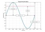
1. The peak or amplitude is valuable for shock events but it doesn’t take into account the time duration and thus the energy in the event.
2. The same is true for peak-to-peak with the added benefit of providing the maximum excursion of the wave, useful when looking at displacement information, specifically clearances.
3. The RMS (root mean square) value is generally the most useful because it is directly related to the energy content of the vibration profile and thus the destructive capability of the vibration. RMS also takes into account the time history of the wave form.
Vibration is an oscillating motion about an equilibrium so most vibration analysis looks to determine the rate of that oscillation, or the frequency. The number of times a complete motion cycle occurs during a period of one second is the vibration’s frequency and is measured in hertz (Hz). For simple sine waves the vibration frequency could be determined from looking at the waveform in the time domain; but as we add different frequency components and noise, we need to perform spectrum analysis to get a clearer picture of the vibration frequency.
Fast Fourier Transform (FFT)
FFT Background
Any waveform is actually just the sum of a series of simple sinusoids of different frequencies, amplitudes, and phases. A Fourier series is that series of sine waves; and we use Fourier analysis or spectrum analysis to deconstruct a signal into its individual sine wave components. The result is acceleration/vibration amplitude as a function of frequency, which lets us perform analysis in the frequency domain (or spectrum) to gain a deeper understanding of our vibration profile. Most vibration analysis will typically be done in the frequency domain.
Fourier analysis works by “testing” for the presence of each frequency component. A discrete Fourier transform (DFT) multiplies the raw waveform by sine waves of discrete frequencies to determine if they match and what their corresponding amplitude and phase are. A fast Fourier transform (FFT) is just a DFT using a more efficient algorithm that takes advantage of the symmetry in sine waves. The FFT requires a signal length of some power of two for the transform and splits the process into cascading groups of 2 to exploit these symmetries. This dramatically improves processing speed; if N is the length of the signal, a DFT needs N2 operations while a FFT needs N*log2(N) operations. So for example, let’s take a signal length of 1024 (210); the DFT needs 1,048,576 operations compared to the much more efficient FFT and its 10,240 operations. Although the execution time of an FFT will be fastest when the signal length is some power of 2, today’s computing power and modern FFT algorithms make this time difference insignificant.
The number of discrete frequencies that are tested as part of a Fourier transform is directly proportional to the number of samples in the original waveform. With N being the length of the signal, the number of frequency lines or bins is equal to N/2. These frequency bins occur at intervals (∆f) equal to the sample rate of the raw waveform (Fs) divided by the number of samples (N), which is another way of saying that the frequency resolution is equal to the inverse of the total acquisition time (T). To improve the frequency resolution, you must extend the recording time.

The lowest frequency tested is 0 Hz, the DC component; and the highest frequency is the Nyquist frequency (Fs/2). Windowing can be used to scale the frequency range of interest and manipulate the frequency bin width. There’s a lot that goes into understanding how windowing works and how to choose the right function for your application;Let’s dive into some examples to understand how spectrum analysis can be used for your vibration testing application!
Constructed Sine Wave and FFT Example
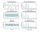
To illustrate how an FFT can be used, let’s build a simple waveform with and use an FFT for vibration analysis. This constructed waveform will consist of three different frequency components: 22 Hz, 60 Hz, and 100 Hz. These frequencies will have an amplitude of 1g, 2g, and 1.5g respectively. The following figure shows how this waveform looks a little confusing in the time domain and also illustrates how the signal length affects the frequency resolution of the FFT. Again, the MATLAB script which generated this data is available to download.
If we sample this wave at a 500 Hz rate (500 samples per second) and take an FFT of the first 50 samples we’re left with a pretty jagged FFT due to our bin width being 10 Hz (Fs of 500 divided by N of 50). The amplitude of these frequency components are also a bit low. But if the range is extended to the first 250 samples as shown then the FFT is able to accurately calculate both the frequency and amplitude of the individual sine wave components.
Not that the “pure” waveform didn’t look confusing enough in the time domain; but if broadband noise is added as shown in the bottom plots then the waveform becomes even less distinguishable. This is the power of an FFT, it is able to clearly identify the major frequencies that exist to help the analyzer determine the cause of any vibration signal.
Real World FFT and Spectrogram Examples
Vibration Analysis of a Car Engine
In real world applications there will typically be many different frequency components of a vibration profile as well as mechanical and electrical noise. Let’s look at some data taken on a passenger car engine while it was idling and do some vibration analysis. This data was generated with a Slam Stick vibration data logger as part of a how-to video series if you’re interested in some more details about the test setup.

We can use spectrum analysis of the vibration profile to indicate what the engine’s crank shaft rotation speed was. This is a 4-cylinder 4-cycle engine. The engine operates with two pairs of pistons moving out of phase with each other and two piston combustions per crank shaft rotation; so the dominant frequency of the engine’s vibration will be twice the crank shaft rotation speed (here’s a nice video on how a 4-stroke engine works). In the FFT there is clearly a dominate frequency at 30 Hz or 1,800 RPM which tells us that at idle the crank shaft is rotating at 900 RPM (or 15 Hz) where there is also a peak in the FFT. The use of an FFT in our vibration analysis gave clues on what was causing the measured vibration.
In many applications the vibration frequency will change with time and you can run into trouble if you only look at the FFT. Let’s zoom out of the area where the car engine is running at a relatively fixed rate, and compute an FFT of the entire signal. In this test the engine sat off for a period of time, idled, then the engine was revved before letting it idle again and finally turning it off. The vibration frequency changed pretty dramatically throughout the test; but the FFT doesn’t capture that. We know from the previous plot that when it was idling there was a fairly significant dominate vibration frequency of 30 Hz; but this peak gets muted when you try and look at the FFT of a changing vibration environment.
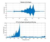
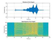
In this example, and others where the vibration frequency changes with time, we need a spectrogram. A spectrogram works by breaking the time domain data into a series of chunks and taking the FFT of these time periods. These series of FFTs are then overlapped on one another to visualize how both the amplitude and frequency of the vibration signal changes with time. Turn this three dimensional surface plot of FFTs on its side, add a color scale to represent the amplitude (often works best when you look at the color/amplitude on a logarithmic scale) and you’re left with a spectrogram!
Back to that car engine example where the engine was revved for a bit. The spectrogram shown below illustrates how the dominate frequencies change with time in relation to when the car engine was idled and revved. Using a spectrogram the analyzer gains a much deeper understanding of the vibration profile and how it changes with time.
Vibration Analysis on the Exterior of an Aircraft during Climb
A spectrogram doesn’t have to be viewed in two dimensions. In the below example I kept the surface plot in the three dimensional view. This is from data taken by a Slam Stick on the outside of an aircraft as it climbed from 23,000 ft to 40,000 feet. The temperature also dropped from 14°C to -31°C (58°F to -24°F) during the test.
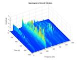
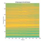
These three dimensional surface plots look pretty cool; but I think that the 2D view better illustrates how the spectrum changes with time as shown below. I wish I could say more about this data and the exact application; but this vibration data was acquired testing our aerospace customer’s proprietary system. The vibration data is really interesting though, and illustrates how enjoyable vibration analysis can be!
Vibration Analysis on a Semi-Trailer Truck during Transit
Now let’s quickly take a look at some data I gathered with our Slam Stick vibration loggers as part of a vibration analysis and energy harvesting study. We had a customer interested in harvesting energy on his trailer bed during shipments to power an asset tracking device using our piezoelectric energy harvesters. Below is an excerpt of the data with a spectrogram, the raw data can be downloaded by clicking the link at the end of this post.
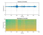
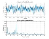
The spectrogram helps us see that that there is definitely some interesting vibration content; and there appears to be a fairly consistent signal around 25 Hz (it’s a must to have a relatively consistent vibration frequency for vibration energy harvesting). We can use an FFT to take a closer look at the vibration profile during a time period where there isn’t a shock, shown below.
The FFT reveals a modest peak around 27 Hz; but the vibration in this environment is still mostly dominated by “random” vibration levels which brings us to how and why PSDs are used in vibration analysis.
Power Spectral Density (PSD)
What is a PSD?
A lot of vibration in the real world, especially during transit, can be called “random” vibration because it is motion at many frequencies at the same time. FFTs are great at analyzing vibration when there are a finite number of dominant frequency components; but power spectral densities (PSD) are used to characterize random vibration signals. A PSD is computed by multiplying each frequency bin in an FFT by its complex conjugate which results in the real only spectrum of amplitude in g2. The key aspect of a PSD which makes it more useful than a FFT for random vibration analysis is that this amplitude value is then normalized to the frequency bin width to get units of g2/Hz. By normalizing the result we get rid of the dependency on bin width so that we can compare vibration levels in signals of different lengths.
PSDs and Vibration Test Standards
Because of how PSDs cancel out the effect of bandwidth of a frequency spectrum, many test standards will describe their vibration environment with a PSD. Let’s go through an example from MIL-STD-810G. Figure 514.6C-5 (page 312) describes the typical acceleration levels that jet aircraft cargo are exposed to as shown below.
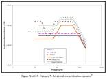
If you were developing something for the government that was going to be transported with a jet aircraft, you would be required to do some testing on your device/equipment to prove it can survive prolonged exposure to those vibration levels. Most shaker control systems will have these exposure profiles built in but they can also be constructed easily given some known PSD levels and rise/decline rates. Let’s take a look at some data captured by a Slam Stick X when it was being excited with these vibration levels; all this data is available to download.
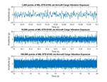
Obviously the raw data in the time domain doesn’t tell us much although I was admittedly surprised by the nearly 20g amplitude of the vibration. Let’s do some vibration analysis and compute both FFTs and PSDs of these signals to see how the signal length affects the amplitude for the FFT but not the PSD.
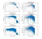
The red lines in the PSD are the input error bounds that the shaker is trying to keep the signal within. As you see, the PSD of different signal lengths just fills in this area but the amplitude doesn’t change overall. The FFT amplitude however shifts down as the bandwidth is increased. The PSD amplitude does not shift because it is normalized to the frequency bin width. This normalization that occurs in a PSD calculation makes it so much more desirable to be used when analysing random vibration signals.
Vibration Analysis of the Seat on a Commercial Airline
Now let’s put ourselves in the shoes of someone buying equipment to be integrated into a larger system. We will want to make sure this equipment can handle the vibration levels in this environment so we may require a test organization to quantify that environment. I used a Slam Stick recently on a commercial flight to do just this, but I wanted to understand what type of vibration levels us humans were exposed to by measuring the seat in front of me. Check out the data below along with a PSD (again this is all available to download).
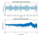
There is definitely a resonance of that seat around 250 Hz; but there is surprisingly steady broadband vibration of 10-5 g2/Hz from 1 Hz to 1 kHz. Now if I was designing a system to operate on/in that airline seat, I could use this PSD to program an exposure profile in our laboratory shaker. Then I’d be able to do some in-house testing ahead of a field test; and because we measured the actual data in the actual environment, we’d have confidence that our system can survive. It’s incredibly valuable to go out and actually measure the environment than to simply rely on some test standard. These test standards will recommend using the standard’s data as a guide; but they typically try and encourage the engineer to go out and get the actual vibration data. Nothing beats the real data!
Summary
FFT
The fast Fourier transform (FFT) is an efficient algorithm used to compute a discrete Fourier transform (DFT). This Fourier transform outputs vibration amplitude as a function of frequency so that the analyser can understand what is causing the vibration. The frequency resolution in an FFT is directly proportional to the signal length and sample rate. To improve the resolution the time of the recording must be extended; but be careful of a changing vibration environment.
Spectrogram
A spectrogram takes a series of FFTs and overlaps them to illustrate how the spectrum (frequency domain) changes with time. If vibration analysis is being done on a changing environment, a spectrogram can be a powerful tool to illustrate exactly how that spectrum of the vibration changes.
PSD
A power spectral density (PSD) takes the amplitude of the FFT, multiplies it by its complex conjugate and normalizes it to the frequency bin width. This allows for accurate comparison of random vibration signals that have different signal lengths. For this reason, PSDs are typically used to describe random vibration environments like those specified in military and commercial test standards.
Getting the Vibration Data
Before you can get started with your vibration analysis, you’ll need to gather some vibration data! If you haven’t gotten that far, explore some vibration measurement options; and if you’re going the route of accelerometers, make sure you select the right accelerometer type.
