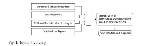
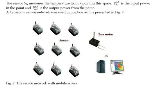
The chapter theme results at the crossroads of some major scientific and technical domains: modern intelligent wireless sensor networks, distributed parameter systems, multivariable linear and non-linear estimation techniques, especially using artificial intelligence tools and virtual instrumentation (Tubaishat & Madria, 2003), (Giannakis, 2008), (Kubrulsky & de S. Vincente,  1977),  (Volosencu,  2008).  And,  an  important  application  is  fault  detection  and diagnosis in system monitoring (Chiang et. al., 2001). This modern concept involving may be represented in Fig. 1.

The  domain  of  system  identification  may  be  developed  today  using  the  powerful  tool represented by the intelligent sensor networks, placed in real distributed parameter systems. Wireless sensor networks (Akyildiz, F. et. al, 2002) may be seen as a collection of numerous sensor  nodes,  each  with  sensing  (temperature,  humidity,  sound  level,  light  intensity, magnetism,  acceleration  etc.)  and  wireless  communication  capabilities,  providing  huge opportunities  for  monitoring  and  mathematical  modeling  of  the  time-evolution  of  the physical quantities under investigation. Sensor networks have proved their huge viability in the real world in the last years (Feng et. al. 2002). One of the important problem related to the  usage  of  wireless  sensor  networks  in  harsh  environments  is  the  identification  of  the states  of  the  physical  variables  in  the  field,  based  on  the  measurements  provided  by  the sensors  (Novak  &  Mira,  2003),  (Pottie  &  Kaiser,  2000),  (Tong  et.  al.,  2003),  (Zhang  et  al.,2005).The modern intelligent sensor networks, with hundred and thousands of ad-hoc tiny sensor nodes spread across a geographical area, may be seen as a “distributed sensor, which may be  placed  in  the  field  of  the  distributed  parameter  systems.  The  sensor  network,  as  a “distributed  sensor”,  allows  the  usage  of  multivariable  estimation  techniques,  in  different ways:  classical  linear  methods  of  modeling  or  methods  based  on  artificial  intelligence  for complex non-linear systems. As smart and small devices the modern sensors are capable to be implemented in large distributed parameter systems.

As  an  example  of  distributed  parameter  system  with  large  application  in  practice  the process  of  heat  conduction  is  presented.  Other  applications  are  presented  in  literature (Rosculet & Craiu, 1979), (Basmadjian, 1999).

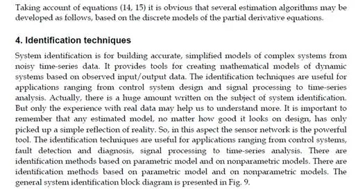
The identification techniques (Ucinski, 2004), (Banks & Kunish, 1989), (Sjoberg, et. al., 1997), (Zhu et. al., 2007) are useful for applications ranging from control systems, fault detection and diagnosis, signal processing to time-series analysis. The  artificial  intelligence  tools  (Chairez  et  al.,  2009),  (Jassar  et.  al.,  2009)  may  be  used  for identification  of  nonlinear  complex  systems  as  the  distributed  parameter  systems  are. ANFIS (Roger Jang, 1993), (Depari et. al., 2005), (Hou & Li, 2006), (Mellit et. al., 2007) as a method for non-linear system identification is a powerful tool to estimate future behavior in distributed parameter systems from acquired data obtained using wireless sensor connected in a distributed network placed in the field.The chapter presents a short survey of some results obtained in the study of using of sensor networks   with   multivariable   estimation   techniques   for   distributed   parameter   system identification.  Sensor  network  topics,  sensor  network  architectures  and  sensor  network applications  are  presented.  Starting  from  the  measurements  collected  by  the  sensor  nodes inside   an   investigated   distributed   parameter   systems,   this   chapter   offers   an   efficient methodology  for  identification  with  linear  and  non-linear  time  series.  Some  estimation algorithms  and  a  method  for  monitoring  distributed  parameter  systems  based  on  sensor networks    and   the    adaptive-network-based    fuzzy    inference    scheme    are    presented (Volosencu,  2010).  The  chapter  presents  an  application  of  a  multivariable  auto-regression estimation technique for estimation of heat transfer in space. A case study of temperature flow for a parabolic equation is analysed, based on these approach. Limited  resources  in  terms  of  computational  power,  energy,  memory  and  bandwidth impose heavy constraints on functionality of an effective malfunction detection system. For this reason these algorithms are designed and suitable for execution on the base station level and,  by  this,  it is  appropriate even  for  large-scale  sensor  networks.  Sensor  networks  have proved their huge viability in the real world, being just a matter of time until this kind of networks will be standardized and used broadly in the field.

Sensor networks

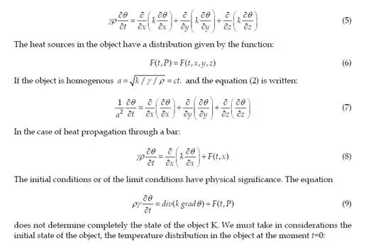
Wireless  sensor  networks  are  extremely  distributed  systems  having  a  large  number  of independent    and    interconnected    sensor    nodes,    with    limited    computational    and communicative potential. The sensors are deployed for data acquisition purposes on a wide range of locations, sometimes in resource-limited and hostile environments such as disaster areas,  seismic   zones,   ecological   contamination   sites   and   other.   In   this   structure   data processing  is  at  the  sensor  level,  data  transmission  is  wireless,  sensing  mechanism  is  not necessarily power supply is not necessarily wireless .Sensor   network   applications   include: 

environmental   monitoring,   civil   infrastructure monitoring,  shared  resource  utilization,  tracking,  perimeter  protection  and  surveillance. Application are in micro-climates, air quality, soil moisture, animal tracking, energy usage,

office  comfort,  wireless  thermostats,  wireless  light  switches.  In  techniques  they  have  as applications  data  acquisition  of  physical  and  chemical  properties,  at  various  spatial  and temporal   scales,   as   in   distributed   parameter   systems,   for   automatic   identification, measurements  over  long  period  of  time.  The  sensor  networks  are  deployed  for  data acquisition   purposes   on   a   wide   range   of   locations,   in   resource-limited   and   hostile environments  such  as  disaster  areas,  seismic  zones,  ecological  contamination  sites.  All applications are distributed parameter systems.

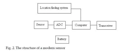
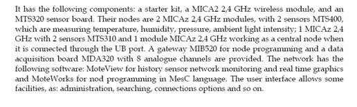
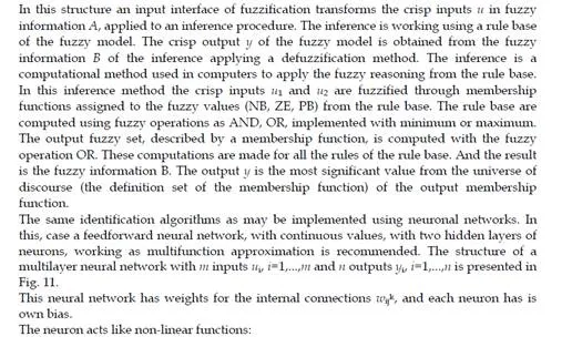
The   modern   sensors   are   smart,   small,   lightweight   and   portable   devices,   with   a communication  infrastructure  intended  to  monitor  and  record  specific  parameters  like temperature, humidity, pressure, wind direction and speed, illumination intensity, vibration intensity, sound intensity, power-line voltage, chemical concentrations and pollutant levels at diverse locations. The sensor number in a network is over hundreds or thousands of ad hoc tiny sensor nodes spread across different area. Thus, the network actively participates in creating  a  smart  environment.  They  are  low  cost  and  low  energy  devices,  realized  in nanotechnology.  With  them  we  may  developed  low  cost  wireless  platforms,  including integrated radio and microprocessors. The sensors are adequate for autonomous operation in  highly  dynamic  environments  as  distributed  parameter  systems.  We  may  add  sensors when they fail. They require distributed computation and  communication protocols. They assure scalability, where the quality can be traded for system lifetime. They assure Internet connections via satellite. The structure of a modern sensor (Akyildiz, F. et. al, 2002), (Pottie& Kaiser, 2000), (Tubaishat & Madria, 2003) is presented in Fig. 2.

The dimension of such a sensor is comparable with a small coin. The sensors are characterized by: a robust radio technology, cheap and energy efficient processors, lifetime energy source, on-board  memory,  flexible  I/O  for  various  sensors,  common  highly  available  components, efficient  resource  utilization  –  currently  uses  10  µA  average,  high  modularity,  flexible  open source platform. Some examples of technical data are: 128 KB instruction EEPROM, 4 KB data EEPROM, 512 KB External Flash Memory, radio with 38 K or 19 K baud, at 900MHz, LEDs, µP at   7,3   MHz,   JTAG,   programming   board,   ISM   Bands:   433-434,8   MHz   Europe,   power consumption:  16  mA  Tx,  9  mA  Rx,  2  µA  sleep,  transmission  range:  1m,  off  the  floor  100m range, ground level 10 m range, interface block data to laptop, GPS, cost: $ 95.Sensor  are  developed  to  measure:  temperature,  humidity,  pressure,  wind  direction  and speed,  illumination  intensity,  vibration  intensity,  sound  intensity,  acceleration,  power-line voltage, chemical concentrations and pollutant levels at diverse locations and others. All are variables in distributed parameter systems. Hundreds or thousands of ad-hoc tiny sensor nodes spread across a geographical area form the  basis  of  a  sensor  network.  Sensor  nodes  collaborate  among  themselves  to  establish  a sensing network. The sensor network provides access to information anytime, anywhere, by collecting, processing, analyzing and disseminating data. The network actively participates in creating a smart environment. Sensor network is working as a distributed sensor.

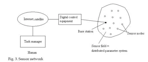
The  constructive  and  functional  representation  of  a  sensor  network  is  presented  in  Fig.  3 (Akyildiz, F. et. al, 2002), (Pottie & Kaiser, 2000), (Tubaishat & Madria, 2003).

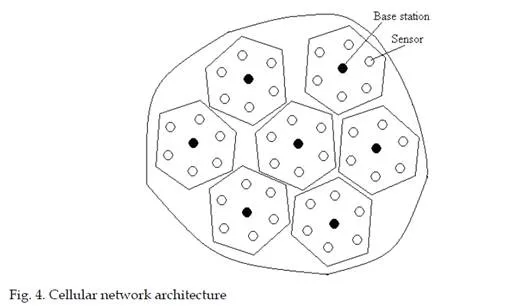
The  sensor  networks  have  different  structures.  The  star  networks  (point-to-point),  are networks in which all sensors are transmitting directly with a central data collection point. The  mesh  networks  are  networks  in  which  sensors  can  communicate  with  each  other.  In mesh networks sensor nodes can relay messages from other sensor nodes, there is no need for   repeaters.   Software   controls   the   flow   of   messages   through   network   with   self- configuration. New nodes automatically detected and incorporate. Advantages of the mesh structures are: robustness, easily deployed, no RF site surveys needed, no repeaters needed, easily expanded.In  the  field  of  sensors  networks  some  topics  are  involved,  like:  development  topics: deployment,  localization,  synchronization,  calibration;  wireless  communication:  wireless radio, characteristics, MAC protocols, link layer techniques, power control; sensor network architecture;  networking  topics:  topology  control,  data  gathering,  network  monitoring, network  coding;  data-centric:  routing  and  aggregation,  querying  and  data  basis,  storage; hardware;  software;  security.  Standards  and  protocols  are  imposed  for  sensor  networks development. Different structure may be uses in practice, for example. The sensor network may be static or  mobile.  For  a  static  case  each  sensor  node  knows  its  own  location,  even  if  they  were deployed via aerial scattering or by physical installation. If not, the nodes can obtain their own  location  through  the  location  process.  Moreover,  all  the  sensors  passed  a  one-time authentication procedure done just after their deployment in the field. The sensor nodes are similar in their computational and communication capabilities and power resources to the current generation sensor nodes. Every node has space for storing up to hundreds of bytes of  keying  materials  in  order  to  secure  the  transfer  of  information  through  symmetric cryptography. There is a base station into the network, sometimes called access point, acting as a controller and also as a key server. It is assumed to be a laptop class device and it is supplied with long-lasting power. An example of a wireless cellular network architecture is presented in Fig. 4.

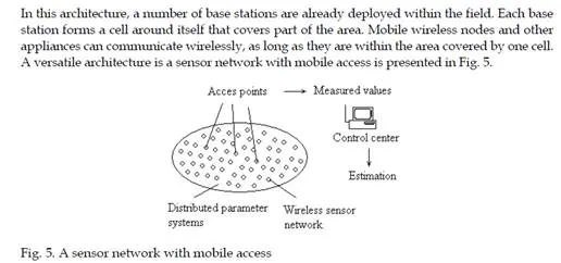
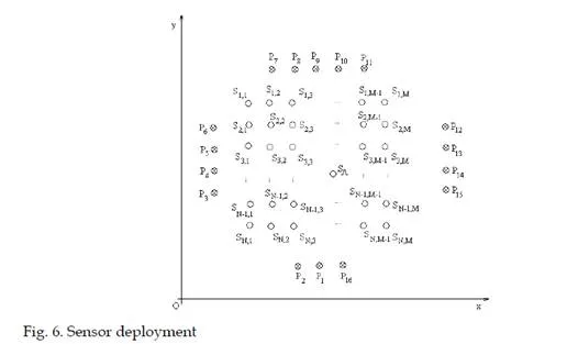
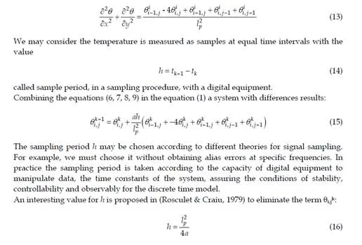
This  structure  used  for  large-scale  sensor  networks.  The  main  difference  related  to  the cellular network architecture is that base stations are considered to be mobile, so each cell has varying boundaries which implies that mobile wireless nodes and other appliances can communicate wirelessly, as long as they are at least within the area covered by the range of the   mobile   access   point.   Multiple   sensor   nodes   can   detect   an   event   situated   in   the surrounding area, so redundancy of sensor networks is assured. In the next paragraph we presents  some  examples  of  such  distribute  parameter  systems  with  their  mathematical models with partial derivative equations.The space model of the sensor deployed in the field with the heat sources is presented inFig. 6.

Distributed parameter systems

The distributed parameter systems, opposed to the lumped parameter systems, are systems whose  state  space  is  infinite  dimensional.  An  object  whose  state  is  heterogeneous  has distributed parameters. Such a system is described by partial differential equations. Partial differential   equations   are   used   to   formulate   problems   involving   functions   of   several variables,  such  as  the  propagation  of  sound  or  heat,  electrostatics,  electrodynamics,  fluid, flow, elasticity. Distinct physical phenomena have identical mathematical formulations, and the  same  underlying  dynamic  governs  them.  One  of  the  most  important  domain  of applications  of  the  partial  differential  equations  is  the  process  of  heat  conduction,  with propagation  of  heat  in  anisotropic  medium:  propagation  of  heat  in  a  porous  medium, transference  of  heat  in  semi-space  compound  by  two  materials  submitted  to  heating, processes of transference of heat between a solid wall and a flow of hot gas, estimation of the  temperature  field  in  space  with  fissured  zone  having  the  form  of  a  circular  disc. Applications related to electricity domain are: the propagation of electric current in cables, the heating of the electrical contacts. In the field of motion of fluid there are: plane motion of viscous  fluids,  running  of  viscous  fluids  in rectilinear  tube,  computation of  losses  of non- stationary  heat  in  subterranean  pipe,  running  of  gases  in  water  main.  The  processes  of cooling and drying: cooling of clap, cooling of a sphere, drying of wood pieces, drying in vacuum. Phenomenon of diffusion: diffusion flow in a heavy sphere for chemical reactions happening with finite spit on the sphere surface, the flames diffusion, which appears to the beginning  of  a  tube,  repartition  density  of  particles  loading  by  the  meteorites.  Other applications  are:  estimation  of  the  ice  height  covering  the  snow  the  arctic  seas,  motion  of underground waters, alloy of heavy fusible particles, investigation of the wave close to the single  point  of  the  board  of  a  plane  plate,  the  growing  of  the  gas  particles in  a  fluid, substances  combustion,  the  temperature  modification  in  the  air  mass.  (Rosculet  &  Craiu,1979), (Basmadjian, 1999).

Processofheatconduction

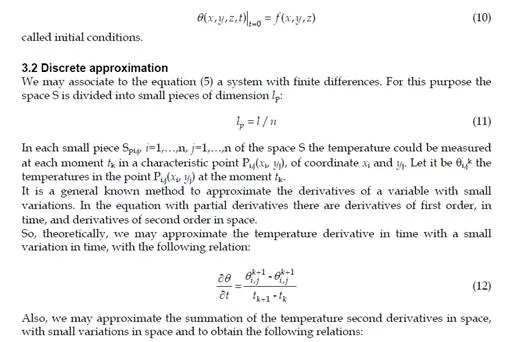
Let it be an object of a volume V ⊂R3  . The frontier of dominium V is a surface S, formed by a finite number of smooth surfaces.

Let it be θ(P, t) the function of the object’s temperature, at the time  moment t,  where  P∈V is a point in the volume V. If different points of object have different temperatures, θ(P, t)≠ct., then a heat transfer will take place, from the warmer parts to the less warm parts. Let it be a regular surface σ  placed in V, which contains the point  P.  From  the  theory  of  thermal  conductivity  through  the  dσ  in  the  time  dt  a  heat quantity  dQ  is  passing,  proportional  to  the  product  dσ.dt  and  proportion  to  the  function θ(P,t) derivative, along the normal n to the surface σ in the point P:

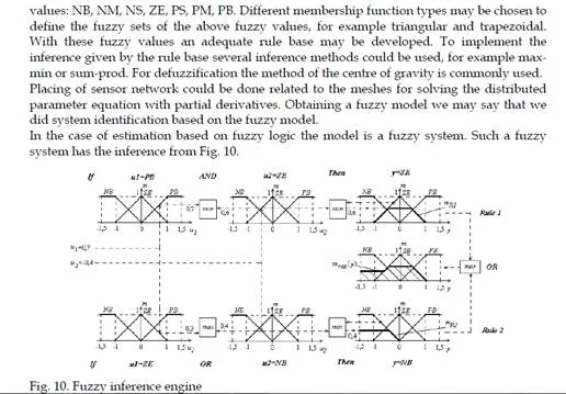
Method for monitoring

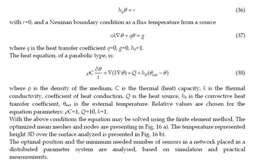
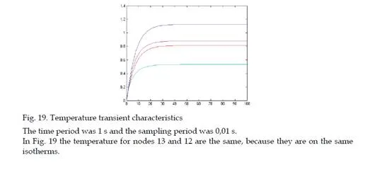
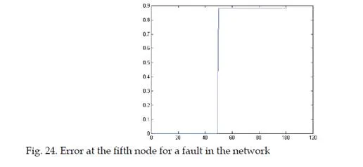
The  following  method  is  according  to  the  objectives  of  monitoring  of  defined  distributed parameter system from the practical application in the real world, as heat distribution, wave propagation.  These  systems  have  known  mathematical  model  as  a  partial  differential equation   as   a   primary   model   from   physics,   with   well-defined   boundary   and   initial conditions for the system in practice. These represent the basic knowledge for a reference model  from  real  data  observation.  The  primary  physical  model  must  be  discretized,  to obtain  a  mathematical  model  as  a  multi  input  –  multi  output  state  space  model.  The unstructured meshes may be generated. The sensors must be placed in the field according to the  meshes  structured  under  the  form  of  nodes  and  triangles.  A  scenario  for  practical applications could be chosen and simulated. The simulation and the practical measurements are producing transient regime characteristics. Those transient characteristics are due to the system dynamics in a training process. In steady state we cannot train the neural model. On these  transient  characteristics,  seen  as  times  series,  the  estimation  algorithms  may  be applied.  ANFIS  is  used  to  implement  the  non-linear estimation  algorithms.  With  these algorithms  future  states  of  the  process  may  be  estimated.  Possible  fault  in  the  system  are chosen  and  strategies  for  detection  may  be  developed,  to  identify  and  to  diagnose  them, base on the state estimation. In practice applying the method presumes the following steps: – placing a sensor network in the field of the distributed parameter system; -acquiring data, in time, from the sensor nodes, for the system variables; -using measured data to determine an estimation model based on ANFIS; -using measured data to estimate the future values of the system  variables;  -imposing  an  error  threshold  for  the  system  variables;  -comparing  the measured  data  with  the  estimated  values;  -if  the  determined  error  is  greater  then  the threshold a default occurs; -diagnosing the default, based on estimated data, determining its place in the sensor network and in the distribute parameter system field.

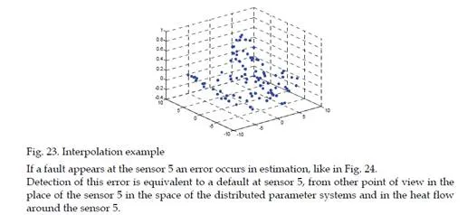
The interpolation techniques may be used for spatial distributed system identification with wireless sensor networks (Volosencu & Curiac, 2009).Considering  the   continuous   development   of   the   wireless  device   technology,   securing wireless  sensor  networks  became  more  and  more  a  significant  task.  One  of  the  important problems that are related to the use of wireless sensor networks in harsh environments is the gap in their security. The strategy on time series predictors based on past and present values obtained from neighboring nodes from this chapter with its estimation algorithms is a basic for discovery of malfunctioning or attacked sensor nodes. Some strategies based on antecedent  values  provided  by  each  sensor  are  presented  for  detecting  their  malicious activity in (Curiac et. al., 2007), (Curiac et. al., 2009), (Plastoi et. al., 2009).

Experimental results

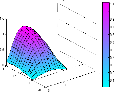
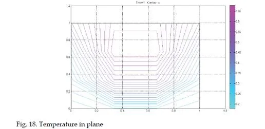
In this chapter a parabolic case study consisting in a heat distribution flux through a plane square   surface   of   dimensions   l=1,   with   Dirichlet   boundary   conditions   as   constant temperature on three margins:

Conclusion

This chapter presents some considerations on time series identification methodology using a wireless sensor network as a complex measurement system. After acquiring the measured values  from  the  area  covered  by  sensor  networks,  some  estimation  techniques  may  be applied. Some auto-regression estimation linear or ANFIS models may be developed. This methodology can be efficiently implemented on sensor network base stations, so there is no need for other hardware resources.A comparison of different identification methods is presented, in order to use the adaptive-network-based  fuzzy  inference.  Some  examples  of  generated  meshes  and  temperature estimates for different numbers of sensor are presented. The main attention is given to the way  of  how  to  chose  the  number  and  the  positions  of  the  sensor  nodes  according  to  the desired accuracy in the identification process.The   chapter   presents   two   algorithms   for   estimation   of   state   variables   in   distributed parameter  systems  of  parabolic  case.  The  algorithms  are  based  on  non-linear  exogenous models  with  regression  and  auto-regression.  Also,  a  method  for  monitoring  distributed parameter  systems  based  on  these  algorithms,  sensor  networks  and  ANFIS  for  non-linear system identification is presented.

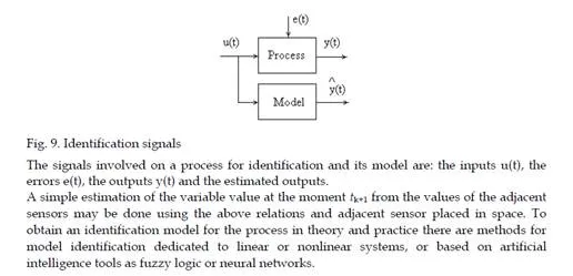
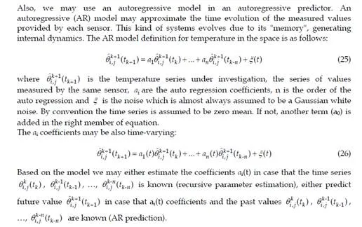
The  sensor  network  is  seen  as  a  “distributed  sensor”.  The  algorithms  are  based  on regression using the values provided by the adjacent nodes of the sensor network and on autoregressive relation with the values from anterior time moments of the same node.

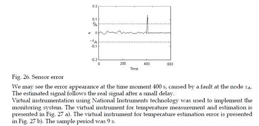
The method described the way how to use all these concepts for fault detection and diagnosis in distributed parameter systems, using the measured values provided by the sensor and the estimated  values  computed  by  the  ANFIS  estimator,  calculating  an  error  and  detecting  the fault  based  on a  decision  taken  after  a  threshold  comparison.  Estimations  methods  may  be applied in the case of discovery of malicious nodes in wireless sensor networks.

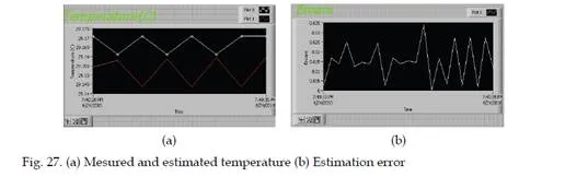
A case study for two algorithms are presented for parabolic type. A comparison between the algorithms is made. Good approximations were obtained. Developing  of  the  algorithms  and  the  method  are  taken  in  consideration  in  the  future,  in other applications, considering all the capabilities of the sensor nodes to measure physical variables.  This  approach  allows  treatment  of  large  and  complex  systems  with  many variables by learning and extrapolation. An interesting application could be the monitoring of  earth  environment  at  low  and  high  altitudes,  based  on  new  types  of  sensor  networks specialized for this purpose. The   implementation   was   made   using   virtual   instruments   of   National   Instruments technology.