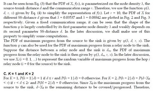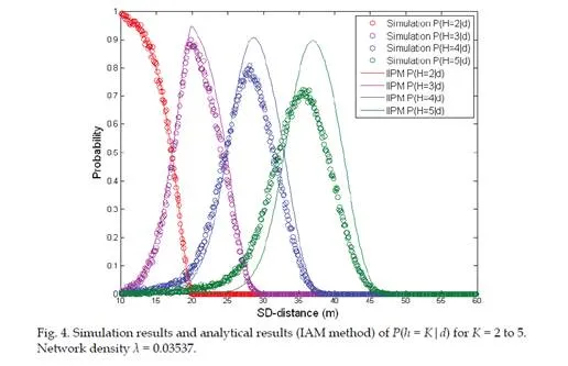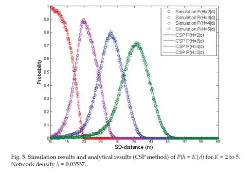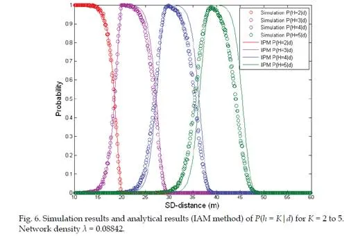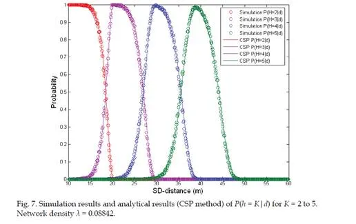
In   large-scale   WSNs   (wireless   sensor   networks),   packets   of   a   source   node   are  often transmitted via multi-hop relays to reach their sink nodes. The hop-count, h, of a sink node is related to a particular hop-count originator (namely the source node) and it is defined as the least number of multi-hop relays required to send one packet from the source to the sink in this chapter. A source node can use a simple controlled flooding to set up the hop-counts relative to itself for all other nodes [1]. Let d denote the Euclidean distance between a source and  its  sink  (the  source-to-sink  distance  is  denoted  as  SS-distance  in  the  sequel),  various statistical  models  that  characterize  the  relationships  between  h  and  d  are  some  of  the fundamental  problems  in  modeling  large-scale  WSNs.  These  results  can  be  applied  to address  many  other  WSN  research  issues  such  as  range-free  localization,  communication protocol design and evaluation, throughput optimization, transmission power control and etc.Given  a  WSN  whose  nodes  are  distributed  randomly  according  to  a  two-dimensional homogeneous Poisson point process of density λ, we investigate two statistical relationships between  hop-count  h  and  SS-distance  d  in  this  chapter.  First  of  all,  we  propose  a  method termed   CSP   (Convolution   of   Successive   Progress)   to   compute   the   K-hop   connection probability for a two-dimensional network. The K-hop connection probability is defined as the conditional probability that a sink has a hop-count h = K with respect to a source given that the SS-distance is d. Mathematically, the K-hop connection probability is defined as the conditional   probability1    P(h   =   K|d).   The   CSP   method   is   also   extended   into   three- dimensional networks.

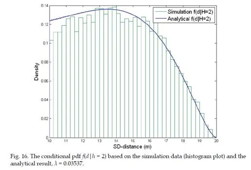
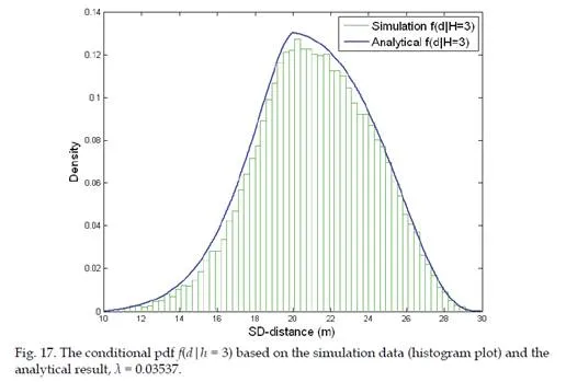
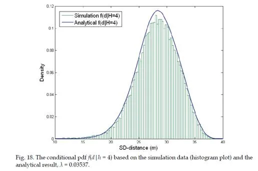
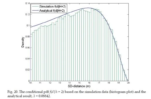
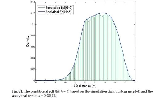
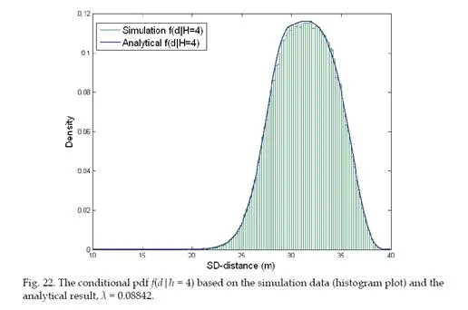
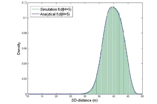
Secondly, based on the results of K-hop connection probability, we also present a method to compute  the  PDF  (probability  density  function)  of  the  SS-distance  d  conditioned  on  hop- count  h  =  K,  namely  the  PDF  of  SS-distance  d  of  all  nodes  with  a  hop-count  h  =  K. Mathematically, this conditional PDF2  is denoted as f(d|h = K). Simulation studies show that the  proposed  methods  are  able  to  achieve  significant  error  reduction  in  computing  these hop-distance   statistics   (i.e.   the   conditional   probability/PDF)   compared   with   existing methods.

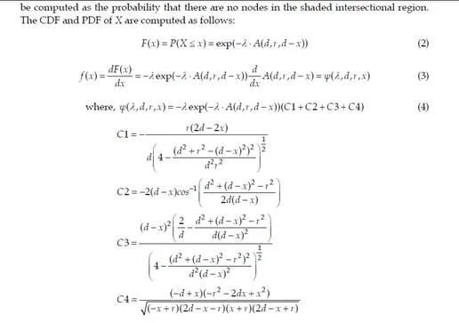
1 Unless otherwise specified, the conditional probability is referred to P(h = K|d) in this paper.

2  Unless otherwise specified, the conditional PDF is referred to f(d|h = K) in this paper.

The  rest  of  the  chapter  is  organized  as  follows.  Section  2  reviews  some  related  works. Section  3  described  the  system  models  used  in  the  analysis.  The  CSP  algorithms  for  both two-dimensional and three-dimensional networks are presented in Section 4. A method of computing the conditional PDF f(d|h = K) is then discussed in Section 5. Section 6 presents simulation results and discussions. Finally, Section 7 concludes the chapter.

Relatedworks

Evaluation  of  various  statistical  models  that  characterize  the  relationships  between  hop- count  h  and  SS-distance  d  are  some  of  the  fundamental  problems  in  modeling  large-scale WSNs. In [2], the solution of the conditional PDF f(d|h = K) for one-dimensional networks is presented. The authors of [3] and [4] derived the conditional probability P(h = K|d) based on the results of [2] for one-dimensional networks. However, only models are provided to the solution of P(h = K|d) in two-dimensional networks. In [5], the exact analytical solution of the  conditional  probability  P(h  =  K|d)  is  derived  for  K  = 1  and  K  =  2  in two-dimensional networks. However, probabilities P(h = K|d) for K > 2 were studied by analytical bounds and extensive simulations. The author of [6] proposed an iterative formulation of P(h = K|d). Though  not  stated  explicitly  in  his  paper,  its  derivation  is  based  on  an  “independent assumption”.  This  independent  assumption  is  then   highlighted  in  [7].  The  analytical solutions proposed in [6] and [7] are the analytical approximations of P(h = K|d) and only converges to the true statistics when the node density λ in the network tends to infinity. Due to  the  complexity  of  two-dimensional  multi-hop  percolation  process,  the  authors  of  [8] proposed a simulation-based attenuated Gaussian approximation to model the conditional PDF f(d|H = K). All previously mentioned results are based on the deployment model that nodes are distributed according to a one-dimensional or two-dimensional Poisson process. The  author  of  [9]  provided  an  analytical  approximation  for  the  probability  of  2-hop connection between two randomly selected nodes in network whose nodes are distributed according to a Gaussian distribution.

Another interesting relationship between hop-count and distance is known as progress per hop. Works related to this are reported in [10] – [13]. The authors of [10] derived a solution for  the  expected  per  hop  progress  in  two-dimensional  networks.  The  expected  per  hop progress problem was also studied in [11] and [12] with different applications in protocol evaluation and localization. The authors of [13] presented an analytic approach to capture statistical bounds on hop-count for a given SS-distance in a greedy routing approach.

The statistical relationships between hop-count and SS-distance can be applied to address many WSN research problems. For example, many range-free WSN localization algorithms employ the principle of hop-count-to-distance transformation to localize nodes. The DV-hop WSN  localization  algorithm  of  [14]  employs  a  heuristics  approach  known as  correction factor to estimate the distance between two nodes based on the hop-count between them. Similar methods are also reported in [15] and [16]. The network throughput problem  and optimal  transmission  radii were  also  studied  in [10]  based on  the  analytical  expression  of expected per hop progress.

System model

In  this  section,  we  discuss  radio  channel  model,  node  deployment  model  and  network topology model used in this chapter.

A.Channel model

As in many WSN literatures, we adopt an unit disk channel model (in some literatures, it is also known as lossless model) in this chapter. A source can communicate directly with all nodes   within   a   disk   centered   at   itself   with   a   communication   range   r,   but   cannot communicate with nodes beyond the disk. The link between a pair of nodes is also assumed to be symmetric, namely, if node A can receive packets from node B directly, then node B also can receive packets from node A directly. The disk model is often used in the theoretical analysis  of  WSNs.  There  are  other  realistic  channel  models  available  (such  as  log-normal shadowing  model  [17]).  These  realistic  channel  models  take  the  random  effect  of  noise, attenuation, shadowing and etc. into consideration. The communication between a pair of nodes  is  thus  characterized  by  PRR  (packet  reception  rate)  or  LP  (link  probability)  rather than  the  absolute  SS-distance.  In  this  chapter,  since  our  study  is  a  general  analysis  of  the statistical relationship between hop-count and SS-distance, we adopt the unit disk channel model so that the radio channel can be regarded as lossless, invariant and homogeneous.

B. Deployment model

We  assume  all  nodes  with  the  same  communication  range  r  are  randomly  deployed  in  a plane  according  to  a  two-dimensional  homogeneous  Poisson  point  process  of  density  λ. Furthermore, we require that all nodes deployed can form a fully-connected network. We make use of the WSN connectivity results presented in [18] to determine suitable values of λ so that all nodes deployed can form a connected network almost surely (probability greater than 0.99).

C. Topology model

Based on the channel and deployment model, we can model the WSN as an undirect graph G. A graph G(V,E) consists a set of vertices (nodes) and edges (links), the set of vertices and edges  are  denoted  by  V  and  E  respectively.  The  shortest  network  path  between  vertices

i  (i  ∈V)  and  vertices  j  (j  ∈V)  is defined  as  the  path  that  travels  through  the  minimum number of edges from i  to j. Therefore, the number of edges traveled is actually the hop- count between i and j. There are many algorithms proposed in the literature to set up the shortest network path in a WSN. These algorithms are out of the scope of this work. In this chapter, we assume that the network paths and the hop-counts between all node pairs have already been set up in advance.

Convolution of Successive Progress

In this section, we propose a method termed CSP (Convolution of Successive Progress) to compute  the  K-hop  connection  probability  in  two-dimensional  WSNs,  i.e.  P(h  =  K|d).  We then  extend  the  CSP  method  to  compute  the  K-hop  connection  probability  in  three- dimensional networks.

A.Problemstatement

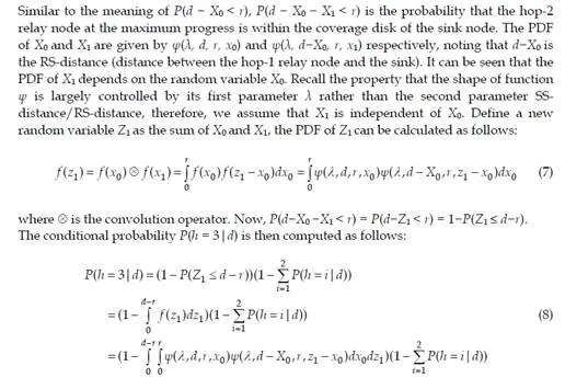
A formal definition of the K-hop connection probability is given in this subsection. Let h and d  denote  the  hop-count  and  distance  between  a  pair  of  source  and  sink.  The  K-hop connection  probability  is  an  important  hop-distance  statistic  and  it  is  defined  as  the probability that the source can reach the sink in K number of multi-hop relays given that the