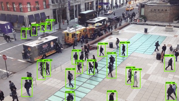
Automatic visual monitoring systems gain more significance as the enhancement of high speed processors that are able to execute the prolonged algorithm efficiently. Video surveillance monitoring systems are typically applied to study human behavior in a crowded situation. It is used to observe posture, movement, trajectories and the interaction between people. For this purpose CCD cameras are installed at many crowded places. Most researchers’ work however is focused on the people classification and the recognition of activities. Human identification is important because of a need of surveillance in the crowded scenes. Group motion tracking is applied to monitor the Groups of People (GOP) as single entities in the global flow rather than monitoring each person individually. It has been studied on the basis of dynamic movement and the surrounding of crowd density which will affect the speed of an individual/group. Large crowd flow perhaps causes deadly accidents if large numbers of GOP smash into each other in narrow passageways, streets or bridges. The system must identify multiple GOP within their global flow according to their Spatio-temporal characteristics. Figure 1 illustrates the density of large crowd flow. The Religious and Sport activities are the application examples. According to Crowd Dynamics Ltd, (Crowd Dynamics Ltd) in the year of 2006, 363 pilgrims lost their lives while performing the Hajj. There are a number of readily available wide area surveillance systems but most of the systems are not suitable for high density crowd monitoring. For safety surveillance of large crowd, there should be a system which can detect and track unstable GOP by careful monitoring of crowd and display results in real- time scenario. And, with the results being displayed in real-time, it will certainly assist the system’s operator to make better decision.

The literature on large crowd flow has got a less coverage from researchers. In the case of large crowd flow scenarios, such as huge flow of peoples as in religious ceremonies or in sport activates, where the flow of crowd have so many individuals or small numbers of groups. On this, commonly used processing techniques cannot be utilized for such uncertain conditions. Dense or huge crowded scenes have so many individuals and groups that pose considerably constraints on these current pre-processing techniques. Ali and Shah (2007) describes crowd flow segmentation.The basic concept which they have used is the Lagrangian particle dynamics to uncover the spatial organization of the flow field generated by crowd flow. Their work is focussed on the crowd flow segmentation, rather than detection and tracking groups of people in a large crowd flow. Their technique is an off-line technique. They generated one mean field from sequence of images to perform the analysis.The main objective of this research work is to develop an efficient monitoring system which can detect and track GOP within a huge crowd, with accurate and computationally efficient manner. A high density crowd flow may exhibits some basic properties of fluid flow. Techniques available in fluid mechanics can be applied to study the flow properties of GOP moving in a large crowd. Previously, crowd flow has been treated as fluid flow to study crowd behavior. The majority of research done in Computational Fluid Dynamics CFD is Eulerian and Lagrangian analysis. Eulerian analyses examine fixed points in space in a fluid flow, while Lagrangian analyses examine individual particles paths.
Technically, global large crowd flow has many similar characteristics as the fluid flow. When coherent structures are studied in terms of its quantities as a consequence of crowd flow trajectories, they are named as Lagrangian Coherent Structures or LCS. The LCS separates the flow of distinct behavior by managing the boundaries where flow field experiencing the different dynamics. This flow boundary in unsteady flows was introduced in a series of papers by Haller (Haller (2001), Haller (2005a) and Haller (2005b)) the boundaries are referred as Lagrangian coherent structures (LCS). New method to evaluate LCS is Finite-Time Lyapunov Exponent field (FTLE) was developed by Shadden (Shadden et al. (2005, Shadden (2006)). Davies et al. (1995) presents the image processing techniques for monitoring crowd behavior. Another idea is to treat the crowd flow as a fluid dynamic, the crowd turbulence is used to study the physics of crowd disasters (Helbing et al. 2007). The density of crowd is an important isotropic quantity that appears to determine the probability of a deadly accident. The crowd flow contains two types of tragedies that is trampling and crushing of pedestrians (Lee and Roger 2005) Trampling occurs when pedestrians are in motion. Crushing usually occur when a moving crowd have a contact with a stationary crowd. The crowd motion organization phenomena such as the directional separation, lane formation, direction towards bottlenecks and stop-and-go type of flow also creates critical conditions. (Helbing et al. 2007b). In crowded scenarios, the focus is on detecting and tracking groups in a global flow rather than in studying individual motion. In this circumstance, Lagrangian Coherent Structure is the most appropriate method. Lagrangian Coherent Structure or LCS is frequently used in fluid mechanics applications in order to distinguish the fluid flow and its associated characteristics. The basic inspiration to used LCS on crowd flow is to treat a flow as a single entity globally, and to track the unstable groups inside the flow. LCS can be computed in different ways, but Finite Time Lyapunov Exponent or FTLE field is the chosen approach (Shadden 2006) since it gives maximum stretching of the nearby particles.
Theoretical background
Lagrangian Coherent Structures LCS
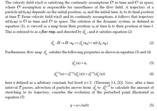
The idea of Lagrangian coherent structures (LCS) stems from dynamical systems which have been extensively used in fluid dynamics analysis. LCS has also been used in the analysis of phase space of systems on the velocity vector field. Coherent motion is defined as a region at which at least one essential flow variable shows important correlation with another variable over a range of space and time Shadden (Shadden et al. 2005, Shadden2006).When coherent structures are studied in terms of its quantities as a consequence of crowd flow trajectories, they are named as Lagrangian Coherent Structures (LCS). The LCS is defined as ridges in the FTLE field. Ridges are the boundaries between the flows of distinct dynamics. The boundary can be determined by tracking flow particles and searching for the material lines that are named separatrices. It has effectively been utilized to partition the flow regions for different dynamics. The technical definition of LCS states that where the gradient of the FTLE field is normal to the eigenvector with the minimum eigenvalue of the Hessian matrix, a scalar field is formed that is the LCS Shadden (2006). The LCS is an invented boundary through which the amount of two or more fluids cannot pass to each other. All the particles within the divided region have similar behavior, known as coherent behavior.In the case of time dependent systems, the crowd flow can be classified as stable and unstable manifolds of hyperbolic fixed points as coherent structures. But typically, one uses the notion of coherent structures in the context of more general flows. Modeling of a dynamical system in a LCS scene gives boundaries in the spatiotemporal separating region. This organization dynamically separates the distinct behavior in the crowd flow which is unseen in the velocity vector field. The boundaries of flow region can be determined by tracking the flow particles during advection which will indicate the material lines. Thus, flow regions with different characteristics would be highlighted. This flow boundary in unsteady flows was introduced in a series of papers by Haller (Haller2001, Haller 2005a and Haller 2005b). These boundaries are referred to as Lagrangian
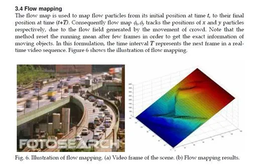
Coherent Structures (LCS).
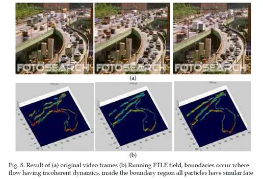
A vector field can be represented as a set of LCS. This LCS has sub regions in which each region contains similar behavior with respect to the crowd flow. The LCS reflects the large scale analysis of a vector field since they are based on the integration of trajectories. At each point in space, the LCS measures the rate of separation of neighboring particle and its trajectories. The LCS of unsteady fields usually distorts and shifts over time, but it still can be recognized. In fluid dynamics, LCS boundaries are the higher ridges of Finite Time Lyapunov Exponent Fields. This ridge refers to material surfaces that get advected with the crowd flow and move towards regions where the flow is separated in positive or negative time. The flow is separated along these boundaries surfaces.The Lyapunov exponent measures the behavior of the flow particles in a dynamical system. It quantifies the exponential rate of convergence or divergence between particles of the neighboring trajectories in a global sense. A positive exponent involves divergence, and a negative one means convergence. Therefore, a system with positive exponents has positive information in that trajectories that are initially close together move at a distance over time. The more positive the exponent, the faster they separate. In the same way for negative exponents, the trajectories move together with each other. A system with both positive and negative Lyapunov exponents is said to be chaotic.
Finite-Time Lyapunov Exponent field (FTLE)
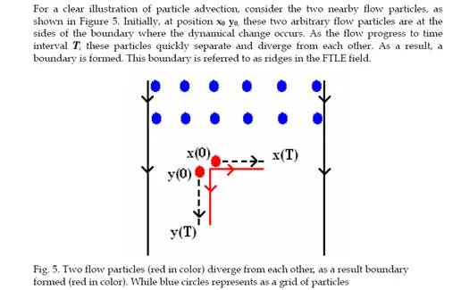
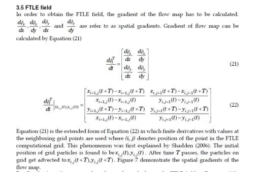
A new method to evaluate LCS is Finite-Time Lyapunov Exponent field (FTLE) was developed by Shadden (Shadden et al. 2005, Shadden 2006). The LCS can be calculated in various ways. One of these methods is based on the FTLE field. It evaluates a value that corresponds to how quickly two imaginary particles would separate from each other as the flow progresses. It measures the maximum linearized growth rate of the distance perturbation between the nearby flow particles over the time interval to its trajectories. In other words, it measures the rate at which two neighboring particles diverge from each other at a given location and time interval. The FTLE differentiates the amount of flow particle stretching about the trajectory over time. It is defined by the local maxima of the FTLE field which specifies regions with distinct dynamics in the flow Haller (2001). Let us suppose that the flow field experienced distinct dynamics in two or more different regions of the same flow. Within each sub region, FTLE contains a coherent motion in the flow that is all the particles inside each region contain a similar behavior which is indicated by the Eigenvalue of λmax (∆) close to zero. The boundary of two flow region contains different dynamics in which particles at these boundaries encloses as incoherent behavior. This condition creates higher Eigenvalue which rises as boundaries in FTLE field. The maximum stretching of particles is given by the square root of the largest eigenvalue. As the stretching is produced by velocity vector field, it would increase exponentially with the time series. The logarithm of the resulting value is computed and additionally normalized by the absolute advection time |T|. This leads to the explanation of the FTLE field. The notation (formulation) of the FTLE will be defined in section 2.3.
The FTLE indicates sections in the flow with different dynamics due to flow particle pairs straddling the edges of the boundary that separate them. This is also to indicate that they are faster than other arbitrary flow particle pairs. Area of maximum material stretching generates local maxima of the velocity field that may specify either local maximal stretching or local maximal shear. Trajectories of the flow particles can be integrated in negative or positive time. This is similar to the scalar parameters in a flow gathering in the coherent structures which can be achieved from the flow vector field. Consequently, FTLE can be calculated by integrating trajectories in backward time (T < 0). The ridges in the FTLE field indicate attracting material lines or attracting Lagrangian coherent structures (attracting LCS) Shadden (2006).Integrating trajectories in forward time (T > 0) produce FTLE ridges that spot the location of distinct flow as material lines, or repelling Lagrangian coherent structures (repelling LCS).These positive-time and negative-time LCS are defined as the boundary between qualitatively different regions in the flow. The integration time can be increased or decreased depending on the amount of feature required from the computation. In addition, the location of the ridge indicating the boundary of the dissimilar flow of crowd does not change.
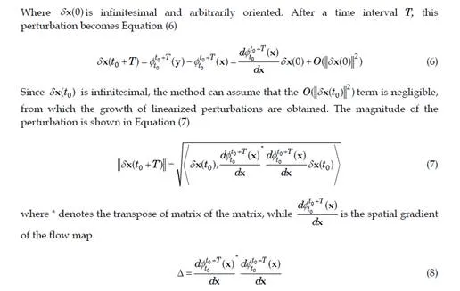
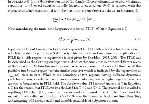
FTLE field with respect to eigenvalue is first given by Shadden [2005, 2006]. The FTLE can be described as the flow region experiences distinct dynamics in two or more different areas of the same flow. Within this each region, we have a coherent motion in the flow i.e. all the particles inside each region contain similar behavior which is indicated by the eigenvalue of λmax(Δ) close to zero. While at the boundary of two regions, having different dynamics, particles at these boundaries having an incoherent behavior, creates higher eigenvalue which
are rise as boundaries in FTLE field. The absolute value |T| is used instead of T in Equation (10) for the reason that FTLE can be calculated for T > 0 and T < 0. The material line is called a repelling LCS when (T>0) over the time interval in forward time. On the other hand the material line is called an attracting LCS (T < 0) over the interval in backward time. Repelling and attracting LCS reveals stable and unstable manifolds of a dynamic system.
Eigenvector parallelism method
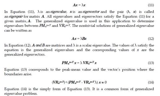
Eigenvalues play an important role in conditions where the matrix is a transformation from one vector space onto itself. Systems of linear ordinary differential equations are the primary examples. The values can correspond to frequencies of vibration, or critical values of stability parameters, or energy levels of atoms it has been discussed in more detail by Moler, C. (2008). As mentioned earlier, LCS can be defined as ridges on the flow field where particles show incoherent behavior. This phenomenon can be explained by the existence of higher eigenvalues at certain region of the flow field. These boundaries separate two regions, and are known as separatrices. Moreover the method requires an approach to extract the information from FTLE field, and identify the precise unstable GOP with respect to its surroundings.In recent years, valuable developments have been made in image segmentation. Several
algorithms have been proposed in which Normalized cut algorithm, is one of the method used for image segmentation first proposed by Shi and Malik (2000). This Normalized cut algorithm is also applicable to perform segmentation on the boundaries of FTLE field. One weakness of this algorithm is that, it process at high computational time to produce results. But in this application, the prime goal is to make the algorithm efficient enough to execute in real-time in real world scenarios. This requires fast running algorithm. In order to overcome this problem generalized eigenvalue is utilized to measure vector parallelism, named this phenomenon as Eigenvector Parallelism. This technique calculates eigenvalue divergence on the FTLE boundaries to identify/segment the exact unstable GOP with respect to their global flow. Consequently, it will differentiate the unstable or hazardous GOP’s boundaries from its flow boundaries with a low computational time.
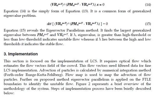
Formulation of Eigenvector Parallelism Method
In Eigenvector Parallelism Method, the technique first correlates the two constitutive mean flow fields RMuu+T and holds the peak-mean value denoted as PMuu+T of the vector field Fuu+T. The characteristic Equation of eigenvalues and eigenvectors is given as:
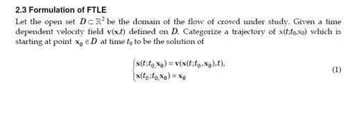
Optical flow
The input prerequisite for FTLE analysis is the velocity vector field. Optical flow, Lucas- Kanade (Lucas & Kanade 1981) technique is used. This is a two frame differential method to estimate motion in a moving object. This method aims to calculate the motion between two image frames which are taken at times t and t + 1 at every pixel location. This method is also frequently known as the differential methods, since it is based on local Taylor series approximations of the image signal. It also uses partial derivatives with respect to the spatial and temporal coordinates.The term optic flow refers to visual phenomenon that has apparent visual motion that can be experienced as an object move through the world. There is a directly mathematical relationship between the magnitudes of the optical flow. If the speed of motion is doubled, the optic flow will also be double. The optical flow also depends on the angle between the direction of view and the moving objects. Advantages of the optical flow algorithm include that it yields a high density of flow vectors. That is, if the flow information missing in inner parts of homogeneous objects is filled-in from the motion boundaries
Smoothing of data
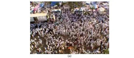
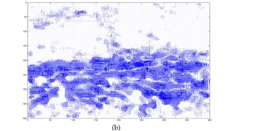
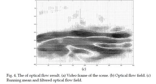
Data smoothing is an important process which contributes to simplify the LCS implementation. It is based on Noise Filtering and Mean value. Figure 3 shows the block diagram of data smoothing process. It is very useful technique which exposes the clear picture of obtained results from optical flow. The optical flow field of crowd motion carries
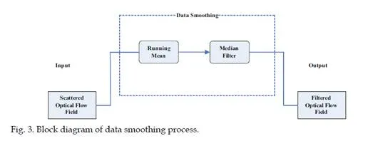
scattered resulting vectors. This is shown in Figures 4 where it is observed that flow vectors of dense crowd have scattered direction and magnitude which is unable to define distinct group behaviors. Data smoothing helps to expose different groups present in the crowd flow by noise reduction and mean flow field.The task for noise reduction is performed by median filtering, which is a non-linear spatial signal enhancement technique. While mean flow field is calculated by taking mean in time series or running mean. It is commonly defined as the continuing calculation. The degree of smoothness can be controlled by adjustment of the neighborhood range or the fitting weights. Fu denoted as optical flow field under observation and its running mean as RMu, here u represents the number of frame in real time video sequence. Running means is programmed in this methodology to reset after a few frames, so that FTLE field can exactly identify the true position of the unstable group.
Advection of particles
In order to detect and track the movement of the flow of crowd, the system launched a Cartesian grid of particles. This movement is known as the advection of particles. These particles are placed on the running mean RMu of flow field Fu, where particles have certain (constant) distance between them. Initially, particle position is x0, at time t. As time T passes, flow of crowd change its position therefore, the optical flow field becomes Fuu+T and its running mean RMuu+T. The final position of particle turn out to be to x(t+T;t,x0). Each particle advection is computed with a forth-order Runge-Kutta-Fehlberg algorithm.
Forth-Order Runge-Kutta-Fehlberg
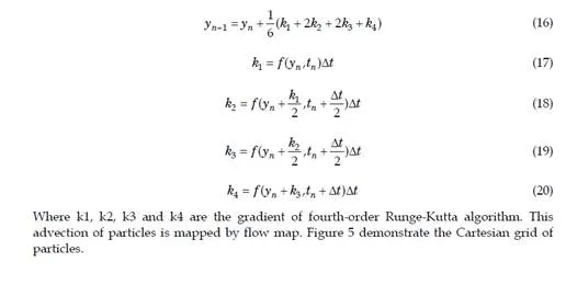
The Runge–Kutta method is an important tool. It is used to perform the approximation of solutions of ordinary differential equations. There are different types of Runge–Kutta methods, classified by how many points are used within each time step. The method applied in the FTLE computation is the 4th Order Runge–Kutta method. This is the most often used method of the Runge-Kutta family. It extends the idea of the mid-point method by using the information.The fourth order Runge-Kutta algorithm requires four gradient or ‘’k’’ terms (as given in equation 16), which can calculate from following equations (17), (18), (19) and (20)
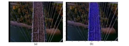
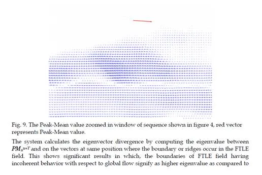
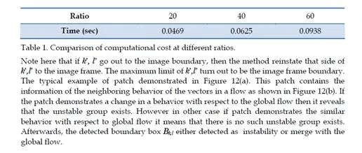
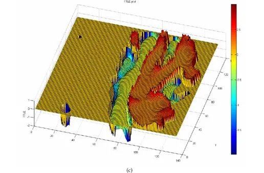
the entire flow FTLE boundaries eigenvalue. This occurs because vectors at the boundaries of FTLE field of unstable GOP have distinct behaviors. Whereas, PMuu+T contains the majority behavior in the global flow. When the system computes the eigenvalue between PMuu+T and the vectors position at boundaries of FTLE field, as a result the stable flow boundaries shows approximately similar characteristic as the peak-mean value. Therefore, the eigenvalue minimize these boundaries, showing evidence of the analogous flow. In other case, unstable GOP boundaries are detected by the FTLE field owing to different dynamics. Vectors at these boundaries give higher eigenvalue when they are computed with PMuu+T. Figure 10 shows the results of Eigenvector Parallelism Method where unstable GOP is detected as higher eigenvalue.
This approach has been tested by changing the direction of unstable GOP on self introduced instability video sequences, and subsequently, observing the imperative results. As the incoherent or unstable GOP changes its flow direction with respect to the global flow, eigenvalue will be increased. Greater the change in direction of flow vector, higher will be the eigenvalue. It will increase until the vectors aligned at the opposite direction as compare to the peak-mean value. In such case where vectors are aligned in opposite directions, a negative eigenvalues in obtained showing unstable GOP. Figure 11 elucidates the negative eigenvalue of GOP, where GOP contains opposite direction with respect to entire flow.
Identification of unstable groups
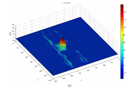
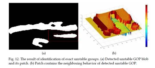
![]() Unstable GOP has dissimilar dynamical behavior and LCS is used to track their boundaries. For the convergence of the detected unstable groups, the technique employed a simple scheme to study the neighboring flow. Let the boundary box of detected unstable group under action denoted by Bk,l, where k, l is its dimensions. At this instance, patch of box Rk’,l’ is launched on the Bk,l, such that size of k’, l’ is determined by a ratio. It can be obtained by taking a ratio between the image frames to the detected object. The resulting ratio will be an integer which will increase the dimension of k’, l’ up to a certain fold. The size of Rk’,l’ is determined by this ratio which is minimizing the computational cost. However different patch size gives different computational cost. A comparison of computational cost is shown in Table 1. In this example, similar detected object is used, in which different ratios are tested in order to calculate the computational costs.
Unstable GOP has dissimilar dynamical behavior and LCS is used to track their boundaries. For the convergence of the detected unstable groups, the technique employed a simple scheme to study the neighboring flow. Let the boundary box of detected unstable group under action denoted by Bk,l, where k, l is its dimensions. At this instance, patch of box Rk’,l’ is launched on the Bk,l, such that size of k’, l’ is determined by a ratio. It can be obtained by taking a ratio between the image frames to the detected object. The resulting ratio will be an integer which will increase the dimension of k’, l’ up to a certain fold. The size of Rk’,l’ is determined by this ratio which is minimizing the computational cost. However different patch size gives different computational cost. A comparison of computational cost is shown in Table 1. In this example, similar detected object is used, in which different ratios are tested in order to calculate the computational costs.
Results and discussion
Group motion detection is a significant tool to study the GOP behavior in a crowded environment. We have utilized LCS to examine GOP in a large gathering. We have tested the algorithm using a range of videos taken from Ali and Shah (2007). This consists of high density crowded scene including videos during Hajj, New York City Marathon and traffic scenes.
Group detection
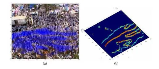
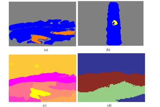
In the sequence entitled ‘Inside Makkah’, as shown in Figure 11(a), a dense and random crowd flow is observed. In this video scene, the direction of global flow is from left to right, three GOP can been seen moving against the direction of the global flow which is detected by Eigenvector Parallelism Method as shown in Figure 11(c). It is noted that two GOP are having hazardous motion dynamics with respect to surrounding crowd because they are disturbing the global flow. It can computed by using method explain in Section 3.6. The third GOP is not hazardous despite having different direction because they are moving independently without propagating inside the moving crowd. Figure 13(a) is the watershed plot used for clear visualization of unstable GOP. Similarly Figure 13(b) is the watershed plot of video sequence shown in Figure 10. Now a comparison of obtained results has been performed with well known methods i.e. K-Mean on optical flow (u,v) field. It is necessary to mention here, that numbers of segments are pre-defined to run this method. Figure 13(c) displays result of K-Mean method which is unable to detect unstable GOP present in the scene although, number of segments has been increased up to 12 in this case. Figure 13(d) shows resulting flow segments of the same video sequence which is under discussion, but this result is obtained from Ali and Shah (2007). Figure 13(d) shows segmentation of crowd according to flow. It is unable to track small groups present at the bottom of the video frame having distinct dynamics. Their method identified the flow (at bottom flow) as single flow and represented it as a single segment. It is because there focus is on flow segmentation not on the tracking of GOP. In contrast, our method detected the flow pattern of crowd as well as tracking small GOP having distinct dynamics with respect to surrounding flow.
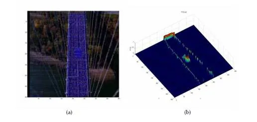
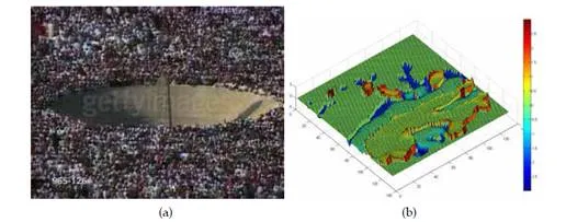
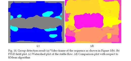
The next result which is discussed here is shown in sequence Figure 1(b). The approach is tested on a video sequence of hurling stones at Jamarat Bridge. This video represented a highly important area where large crowd of people gather to perform a similar task. In the past, most of the deadly incidents occur at Jamarat Bridge due to collision of people in high density crowd. Detection and tracking of GOP having unstable dynamics are challenging task in this video sequence, since the flow pattern is quite complex and density of crowd is very high. The proposed method is able to work and produce results in such a highly dense crowd. The direction of global flow in this scene is from right to left. Few GOP are detected and tracked having different direction. The result of Eigenvector Parallelism Method is displayed in Figure 14(b).Figure 14(c) is the watershed plot used for clear visualization of unstable GOP. The result was then compared with K-Mean methods. In this case K-Mean is unable to segment the crowd flow exactly, due to complexity and density of the scene. In Figure 14(c) three hazardous groups are highlighted below vacuum region (at the bottom) while two GOP are present above vacuum region. While K-Mean method could only detects two GOP at the bottom out of three while merged the upper groups with the global flow as shown in Figure 14(d). This shows the robustness of the proposed Eigenvector Parallelism Method.
Test set
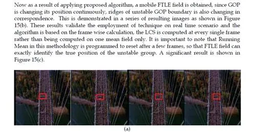
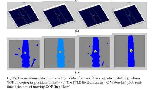
The video sequence of New York City Marathon already used in Figure 10, in which artificial instability was generated by Ali and Shah (2007). In this sequence unstable GOP had different direction with respect to the global flow but GOP was static throughout the video. Now a moving GOP is introduced in the video sequence shown in Figure 15(a), the direction of mobile GOP is from left to right which is changing its position in every incoming frame. This continuous change in position makes the GOP a challenging object to track. This is mathematically described as, Pt = (offset x + fr) + offset y. Where Pt is referred as position of patch (i.e. unstable GOP), fr is number of frame sequence which can be defined as fr= 1, 2, 3….n and offset is value where patch is initially launched.
Algorithm computational time
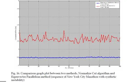
The robustness of the work depends on the fast running algorithm that will run efficiently, in order to do real-time analysis. To apply the Lagrangian technique on the image sequences requires few numbers of frames in reading memory. These frames become the integration length |T| for the algorithm. This requirement indicates that Lagrangian methodology is only applicable for off-line analysis. The solution of off-line analysis problem is solved by MatLab™ M-file and pre-system Simulink™ interface, both simultaneously worked together. Simulink model worked as pre-system, consist of reading frames from data acquisition box and data smoothing. While the M-file worked as post-system, contains of all the methodology of Lagrangian technique. This project is applicable for frame wise analysis rather than estimate one mean field from the integration length |T|. In this formulation, the integration length |T| represents the next frame in real-time videos. The algorithm was implemented, and all analyses have been conducted on a 3 GHz core2duo Pentium IV computer, executing Windows XP. The processing time for a single frame, size of 400×400 RGB image, is approximately 0.5 second that is 2 frames per second. This technique has assumed that the group motion is a slow performing motion because people moving in a large crowded scene. However, the execution time can be increased up to 5 frames per second by reducing the image size. Nevertheless, this will cause a loss of spatial image information.
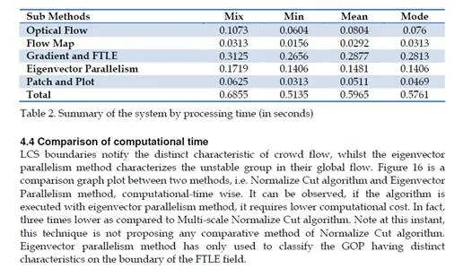
In general Lagrangian sense, taking a denser particle grid will give higher spatial resolutions, which will lead to a higher computation time. If longer time integration is used, more of the boundaries will be exposed. Since flow particles were observed for longer time period consequently more boundaries will be exposed. This methodology cannot make use of longer time integration due to the computational cost restriction. Table 2 shows the computational cost of sub-systems for different sub-methods. Table 2 is computed on the sequence title “Inside Makkah”.
Conclusion
This chapter provides a general framework for group motion detection and tracking in real- time crowded scenarios by using Lagrangian based approach. The main objective of this research is to detect and track Groups of People (GOP) that may create a calamity due to
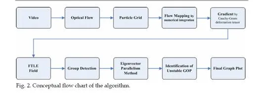
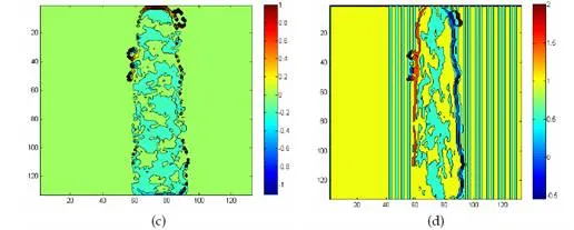
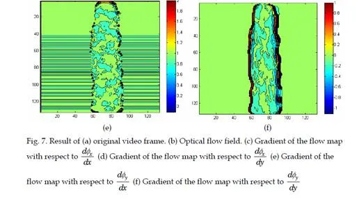
their unstable motion. This objective has been achieved by employing a Lagrangian Coherent structure (LCS). The motivation for using LCS method came from the field of fluid mechanics which is able to reveal the spatial organization of the flow field created by the crowd flow. The Finite Time Lyapunov Exponent (FTLE) Field is one of the most appropriate approaches to obtain the LCS. It measures the maximum divergence between two particles as the flow progresses. At first the optical flow was used to give the flow field on which the system launched a particle grid for tracking the advection of crowd flow. These advected of particles are mapped by flow mapping on which spatial gradient is computed. Finally Finite-time Lyapunov Exponent (FTLE) field is computed on this gradient of flow map. The FTLE field restores the boundaries where the crowd flow experiences the dynamic change. On these boundaries, the system employed a new method of eigenvector parallelism in order to identify the precise unstable groups that are propagating in the global flow. One of the common requirements of the motion detection algorithms in computer vision is the perspective views of camera. In this approach for detection of GOP in a crowded scene, the flow of crowd must be visualized from certain height for the visibility of the spatial organization of the flow. The variability of the image captured will also produce significant noise source to the overall analysis. In this case, stationary camera is used to minimize the capture noise factor. The developed monitoring system successfully tracks a range of objects, which can easily be used for actual monitoring requirements. The method suggested is very robust and can be adapted to various crowded scenarios such as traffic flow and fish schooling, where thousands of objects are involved.