Synthetic Aperture Radar (SAR) systems are all-weather, night and day, imaging systems. Automatic interpretation of information in SAR images is very difficult because SAR images are  affected  by  a  noise-like  characteristic  called  speckle  that  arises  from  an  imaging  device and  strongly  data  and  makes  automatic  image  interpretation  very  difficult.  The  speckle noise   in   SAR   images   can   be   removed   using   an   image   restoration   technique   called despeckling.  The  goal  of  despeckling  is  to remove  speckle-noise  from  SAR  images  and  to preserve  all  image’s  textural  features.  The  statistical  modeling  of  SAR  images  has  been intensively investigated over recent years. In statistical image processing an image can  be viewed  as  the  realization  of  a  joint  probability  density  function.  Since  joint  probability functions have analytical forms and few unknown parameters usually, the efficiency of the denoising algorithm depends on how well the chosen model approximates real data.

The wavelet Daubechies (1992) based despeckling algorithms are proposed in Dai et al. (2004), Argenti  et  al.  (2006),  Foucher  et  al.  (2001).  The  second-generation  wavelets  like  Contourlet Chuna  et  al.  (2006)  have  appeared  over  the  past  few  years.  Despeckling  using  Contourlet transform  Li  et  al.  (2006)  and  Bandelet  Sveinsson  &  Benediktsson  (2007)  transforms  show superior  despeckling  results  for  SAR  images  compared  with  the  wavelet  based  methods. Model based despeckling mainly depends on the chosen models. Bayesian methods have been commonly  used  as  denoising  methods,  where  the  prior,  posterior  and  evidence  probability density functions are modeled. The image and noise models in the wavelet domain are well- defined  using  the  results  in  Argenti  et  al.  (2006),  Gleich  &  Datcu  (2007)  and  the  noise  free image is estimated using a MAP estimate. The speckle noise in the SAR images is considered as  a  multiplicative  noise  Walessa  &  Datcu  (2000),  and  can  be  also  presented  as  a  signal- dependent additive noise Argenti et al. (2006). The log transformed image is modeled using zero  location  Cauchy  and  zero-mean  Gaussian  distributions  in  order  to  develop  minimum means absolute error estimator, and maximum a posteriori estimator. This paper presents the state-of  the  art  methods  for  information  extraction  and  their  comparison  in  efficiency  of despeckling  and  information  extraction.  This  paper  presents  three  methods  for  despeckling and  information  extraction.  The  first  method  is  wavelet-based  despeckling  and  information extraction  method  using  the  General  Gauss-Markov  Random  Field  (GGMRF)  and  Bayesian inference of first and second order. The second and third methods use the GMRF and Auto- binomial  model  with  the  Bayesian  inference  of  first  and  second  order.  The  despeckling performance is compared and the texture parameters estimation is presented.

Synthetic Aperture Radar System

The Synthetic Aperture Radar systems are all weather, day and night monitoring systems, which  use  the  electromagnetic  radiation  for  image  retrieval.  SAR  is  one  of  the  most advanced  engineering  inventions  systems  in  the  last  decade.  Specific  radar  systems  are imaging radars, such as side looking SAR and SAR. Practical restriction to the length of the antenna  resulted  in  very  coarse  resolution  in  the  flight  direction.  Using  a  fixed  antenna, illuminating  a  strip  or  swath  to  the  sensor’s  ground  track,  resulted  in  the  concept  of stripping   mapping.   Modern   phased-array   antennas   are   able   to   perform   even   more sophisticated data collections strategies, as ScanSAR, spotlight SAR, but the strip map mode is the most applied mode on current satellites [1]. The concept of using frequency (phase) information  in  the  radar  signal’s  along-track  spectrum  to  discriminate  two  scatters  within the antenna beam goes back to 1951 (Carl Wiley). The key factor is coherent radar,, where the phase and amplitude are received and preserved for later processing., but long antenna was  required.  The  early  SAR  systems  were  based  on  optical  processing  of  the  measured echoed  signal  using  the  Fresnel  approximation  for  image  formation  and  are  known  as range-Doppler   Imaging  or   polar  format   processing.  The  experience  on  airborne  SAR systems  in  60’s  and  70’s  culminated  in  L-band  SAR  system  Seasat,  a  satellite  launched  in June 1978, primarily for ocean studies, the live time was 100 days, but the imaginary was spectacular, highlighting if geologic information and ocean topography information. Since 1981  Shuttle  missions  carried  SAR  systems.  The  first  instrument  was  the  Shuttle  Imaging radar SIR laboratory and operated for 2.5 days. An improved version of SIRA orbited the Earth  in  1984  and  was  able  to  steer  the  antenna  mechanically  to  enable  different  angels. Cosmos  1870  was  the  first  S-band  SAR  satellite  of  former  Soviet  Union,  launched  in  1987 and  orbited  at  a  height  of  270  km  and  operated  for  2  years,  ALMAZ-1  was  the  second satellite  launched  in  1991  and  operated  for  1.5  years.  First  European  Remote  Sensing Satellite ERS-1 was operational in 1991 and operated until March 2000. Japan started space- borne SAR program in 1992 with JERS in 1992, SIR-C/X-SAR was developed by JPL, DLR and ASI operated with C, L and X band. Canadian Space Agency lunched Radarsat in 1995. A SRTM (Shuttle Radar Topography mission) was carried out between 11 and 23 February 2000.  In  last  decade  many  other  satellites  with  SAR  were  lunched:  Radarsat-2,  ENVISAT, TerraSAR-X, Tandem-X, ALOS, Cosmo-Skymed, SAR lupe and forth coming constellation of Sentinel satellites.

Principles of SAR

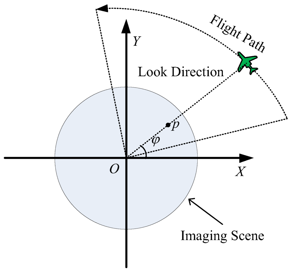
The central idea of SAR processing is based upon matched filtering of the received signal in both the range  and azimuth  directions.  Matched filtering is possible because the acquired SAR   data   are   modulated  in   these   directions   with   appropriate   phase   functions.   The modulation  in  range  is  provided  by  the  phase  encoding  of  transmitted  pulse,  while  the modulation in azimuth is created by the motion in the signal. The point targets are arrayed in  a  Cartesian  type  Coordinate  system  space  defined  by  range,  azimuth,  and  altitude  as analogs  of  x,  y  and  z  directions.  The  altitude  direction  is  omitted  in  the  two-dimensional simulation. The platform in this simulation is an antenna attached to a plane traveling at an orbital velocity, along the azimuth direction and at the midpoint in the flight, the distance to the target equals the range of closest approach or minimum range to target. As an satellite platform is used in the simulation, the curvature of the earth is considered negligible and the orbital velocity is approximately equal to the platform velocity. The transmitted radar signal, x(t), is assumed to be a chirp pulse (linearly frequency modulated signal) given by

areas on the earth’s surface in the same range but in different azimuth, are located on the same azimuth frequency. So, when this frequency is adjusted, the whole target areas with the  same  frequency  (which  means  in  the  same  range)  are  adjusted.  RDA  uses  the  large difference in time scale of range and azimuth data and approximately separates processing in these two directions using Range Cell Migration Correction (RCMC). RCMC is the most important  part  of  this  algorithm.  RCMC  is  performed  in  range  frequency  and  azimuth frequency  domain.  Since,  azimuth  frequency  is  affected  by  Doppler  Effect  and  azimuth frequency is  bonded with Doppler frequency, it is called Range Doppler Algorithm.  RDA can  be  implemented  in  three  different  ways.  But  they  all  have  similar  steps  and  their difference is only in Secondary Range Compression (SRC). The main steps of RDA are: 1- Range  compression  2-  Azimuth  FFT  (transform  to  range  Doppler  domain)  3-  RCMC  4- Azimuth filtering 5- Inverse FFT (return to range azimuth time domain) 6- Image formation. Range compression is implemented using matched filter. The filter is generated by taking the  complex  conjugate  if  the  FFT  of  the  zero  padded  pulse  replica,  where  the  zeros  are added to the end of the replica array. The output of the range matched filter is the inverse transform between range Fourier transformed raw data and the frequency domain matched filter.  Each  azimuth  signal  is  Fourier transformed  via  an  azimuth  FFT  and  RCMC  is performed  before  azimuth  matched  filtering  in  the  range-Doppler  domain.  After  azimuth matched  filtering  of  each  signal  and  azimuth  inverse  fast  Fourier  transforms  (IFFTs),  the final target image is obtained. Fig. 2 shows, real and imaginary part of the received signal, The simulated raw data and its real part and phase are shown in Fig. 3. Fig.4 shows the process of range compression with RCMC and its phase

Image and speckle models

SAR images are affected by a noise-like characteristic called speckle that affects all coherent imaging  systems  and,  therefore,  can  be  observed  in  laser,  acoustic  and  radar  images. Basically,   this   usually   disturbing   effect   is  caused   by   random   interferences,   either constructive  or  destructive,  between  the  electromagnetic  waves  which  are  reflected  from different  scatterers  present  in  the  imaged  area.  SAR  images  appear  to  be  affected  by  a granular  and  rather  strong  noise  named  speckle.  Speckle  becomes  visible  only  in  the detected amplitude or intensity signal. The complex signal by itself is distorted by thermal noise   and   signal   processing   induced   effects   only.   As   a   consequence   of   the   speckle phenomenon, the interpretation of detected SAR images is highly disturbed and cannot be done with standard tools developed for non-coherent imagery. Magnitude and phase of the scatterers  are  statistically  independent,  allowing  to  obtain  the  received  signal  by  a  simple summation  of  the  individual  contributions.  Interactions  between  scatterers  are  neglected.The  phase  of  the  scatterers  is  uniformly  distributed  between  0  and  2π,  i.e.  speckle  is assumed to be fully developed.

SAR image statistics

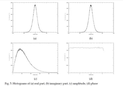
The  SAR  image  is  a  complex  image,  where  the  real  and  imaginary  part  have  Gaussian distribution, with zero mean and its real and theoretical distributions are shown in Fig. 5(a) and 5(b). The amplitude of the SAR image is obtained using the absolute value and can be modeled using Gamma distribution

they  are  able  to  statistically  describe  correlations,  or  even  more  generally,  any  kind  of statistical dependence between neighboring pixels. Furthermore, they are easily applicable within the Bayesian framework. Originating from statistical physics, where they have been used  for  the  study  of  phase  transitions,  they  are  now  widely  employed  to model  two- dimensional  lattices,  such  as  image  data.  In  the  beginning,  the  use  of  Markov  models  in image processing was limited due to the constraint of causality, but after a solution to this problem had been found, they quickly became one of the standard image processing tools. The  information  of  digital  images  is  not  only  encapsulated  in  gray-values  of  individual pixels. More than that, images are usually composed of different regions and features with similar  statistical  properties,  such  as  textures,  lines  and  contours.  As  of  this,  several independently considered pixels usually are not significant to describe all information of a certain image region, but become important by their relations and interactions with pixels in a  neighborhood.  The  characteristics  of  these  local  interactions  between  pixels,  defining different regions of an image, can be modeled by a Markovian formalism, which is suitable for  the  envisaged  framework  of  Bayesian  data  analysis.  The  MRF  model  characterize  the spatial  statistical  dependency  of  2-D  data  by  symmetric  set  called  neighbor  set.  The expression

∑ θr (xs+r  + xs−r )

r∈ζ s

presents  the  sum  of  all  the  distinct  cliques  of  neighboring pixels  at  a  specific  subband.  For  the  first  order  model  of MRF,  a  sum  is  performed  over horizontal  and  vertical  neighboring  pixels.  The  neighbor  set  for  a  first  model  order  is defined as ζ = {(0,1), (0,–1)(1,0), (–1,0)} and for a second model order ζ = {(0,1), (0,–1)(1,0),

(–1,0),  (1,1),  (–1,–1),  (1,–1),  (–1,1)}.  The  MRF  model  is  defined  for  symmetric  neighbor  set, therefore, if r ∈ ζs  then –r ∉  ζs and ζ is defined as ζ = (r : r ∈ ζs) [ (–r : r ∈ ζs). MRF can be described by potential functions working on a local neighborhood due to the Gibbs-Markov

equivalence.   In   principle,   there   are   no   restrictions   to  the   contents  of   these   potential functions. The potentials attached to different cliques do not even have to be stationary but can  vary  throughout  the  image.  For  the  problem  of  image  restoration  or  information extraction, however, a certain number of ”standard” potential functions exist. Local interactions can be described by potentials Vc  for different cliques c. These potentials are a function of the gray-values of the pixels belonging to a clique. Hence, the global energy of the whole image can be written as the sum over all potentials

textures in the real-SAR image. Figs. 9(a)-9(c) show the ratio images of real SAR images. The speckle is well estimated with all presented methods. The MRF based methods are able to extract features parameters. In this case the texture can be extracted using texture models. The texture parameters obtained with the GMRF, ABM and GGMRF models are shown in Figs. 10(a)-10(f), where the horizontal and vertical cliques are shown. The ABM model well models homogeneous and heterogeneous regions, as well it separates different kind of textures, as show the ABM’s texture parameters on Figs. 10(c)- 10(d). The GMRF model is not as efficient as the ABM model in modeling real textures, but it  is  still  able  to  model  homogeneous  and  heterogeneous  regions  and  the  parameters estimated with the GMRF model are shown in Figs. 10(a)-10(b). The wavelet based method has difficulties in modeling textures. This can be the consequence of the linear model used for  the  texture  parameter  estimation.  The  texture parameters  obtained  with  the  GGMRF model are shown in Fig. 10(e)-10(f). The computational efficiency of the proposed methods were tested on real SAR image with 1024 ×1024 pixels and the execution times were 414, 560 and 103 seconds for MAP-GMRF, MAP-ABM and MAP-GGMRF methods.

Conclusion

Presented methods in this paper are based on Markov Random Fields. The efficiency of two methods, which work within the image domain and the wavelet based method is compared. The wavelet-based method gives good results in the objective measurements on simulated data, well preforms in the terms of despeckling, but its ability of information extraction in very poor. The ABM in GMRF based methods well despeckles the real and simulated dataand the ABM gives very good results using real SAR data. The ABM has better ability to separate  blob-like  textures,  which  occur  in  the  real  SAR  images  for  city  areas.  The  GMRF model is more appropriate for the natural textures.