As discussed in the previous part of Lesson 4, the shape of a velocity versus time graph reveals pertinent information about an object’s acceleration. For example, if the acceleration is zero, then the velocity-time graph is a horizontal line (i.e., the slope is zero). If the acceleration is positive, then the line is an upward sloping line (i.e., the slope is positive). If the acceleration is negative, then the velocity-time graph is a downward sloping line (i.e., the slope is negative). If the acceleration is great, then the line slopes up steeply (i.e., the slope is great). This principle can be extended to any motion conceivable. Thus the shape of the line on the graph (horizontal, sloped, steeply sloped, mildly sloped, etc.) is descriptive of the object’s motion. In this part of the lesson, we will examine how the actual slope value of any straight line on a velocity-time graph is the acceleration of the object.
Analyzing a Constant Velocity Motion
Consider a car moving with a constant velocity of +10 m/s. A car moving with a constant velocity has anacceleration of 0 m/s/s.
The velocity-time data and graph would look like the graph below. Note that the line on the graph is horizontal. That is the slope of the line is 0 m/s/s. In this case, it is obvious that the slope of the line (0 m/s/s) is the same as the acceleration (0 m/s/s) of the car.
| Time (s)Velocity (m/s)010110210310410510 |  |
So in this case, the slope of the line is equal to the acceleration of the velocity-time graph. Now we will examine a few other graphs to see if this is a principle that is true of all velocity versus time graphs.
Analyzing a Changing Velocity Motion
Now consider a car moving with a changing velocity. A car with a changing velocity will have an acceleration.
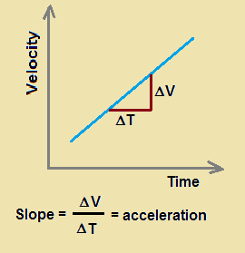
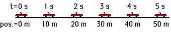
The velocity-time data for this motion show that the car has an acceleration value of 10 m/s/s. (In Lesson 6, we will learn how to relate position-time data such as that in the diagram above to an acceleration value.) The graph of this velocity-time data would look like the graph below. Note that the line on the graph is diagonal – that is, it has a slope. The slope of the line can be calculated as 10 m/s/s. It is obvious once again that the slope of the line (10 m/s/s) is the same as the acceleration (10 m/s/s) of the car.
| Time (s)Velocity (m/s)00110220330440550 |  |
Analyzing a Two-Stage Motion
In both instances above – the constant velocity motion and the changing velocity motion, the slope of the line was equal to the acceleration. As a last illustration, we will examine a more complex case – a two-stage motion. Consider the motion of a car that first travels with a constant velocity (a=0 m/s/s) of 2 m/s for four seconds and then accelerates at a rate of +2 m/s/s for four seconds. That is, in the first four seconds, the car is not changing its velocity (the velocity remains at 2 m/s) and then the car increases its velocity by 2 m/s per second over the next four seconds. The velocity-time data and graph are displayed below. Observe the relationship between the slope of the line during each four-second interval and the corresponding acceleration value.
| Time (s)Velocity (m/s)0212223242546678810 | 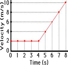 |
| From 0 s to 4 s: slope = 0 m/s/s From 4 s to 8 s: slope = 2 m/s/s |