1)      

b)      Boundary conditions:  

c)      Initial condition: 

d)      Solution: 

2)               Dimensionless heat transfer coefficient

3)                     Dimensionless time also denoted by τ

4)      Note that the characteristic length in the definition of the Biot number is taken to be the half-thickness L for the plane wall and the radius r for the long cylinder and sphere instead of V/A used in lumped system analysis.

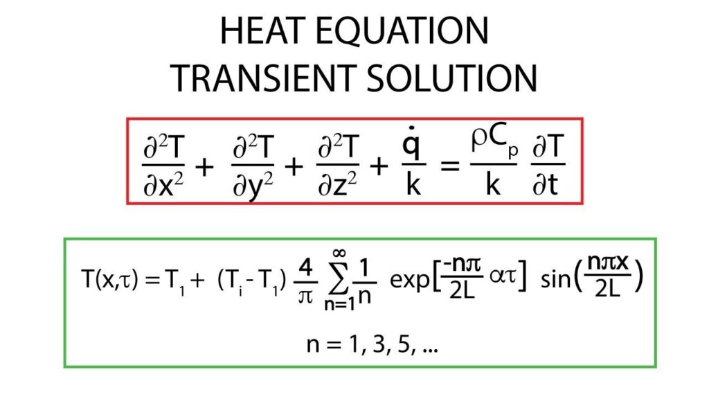
5)      The one-dimensional transient heat conduction problem just described can be solved exactly for any of the three geometries, but the solution involves infinite series, which are difficult to deal with. However, the terms in the solutions converge rapidly with increasing time, and for τ > 0.2, keeping the first term and neglecting all the remaining terms in the series results in an error under 2 percent. We are usually interested in the solution for times with τ >0.2, and thus it is very convenient to express the solution using this one term approximation

6)      Once the Bi number is known, the above relations can be used to determine the temperature anywhere in the medium. The determination of the constants A₁ and λ₁ usually requires interpolation. For those who prefer reading charts to interpolating, the relations above are plotted and the one-term approximation solutions are presented in graphical form, known as the transient temperature charts. Note that the charts are sometimes difficult to read, and they are subject to reading errors. Therefore, the relations above should be preferred to the charts.

a)      The transient temperature charts in for a large plane wall, long cylinder, and sphere were presented by M. P. Heisler in 1947 and are called Heisler charts.

b)      There are three charts associated with each geometry: the first chart is to determine the temperature T_o at the center of the geometry at a given time t. The second chart is to determine the temperature at other locations at the same time in terms of T_o . The third chart is to determine the total amount of heat transfer up to the time t. These plots are valid for τ >0.2.

c)      The use of the Heisler/Gröber charts and the one-term solutions already discussed is limited to the conditions specified at the beginning of this section: the body is initially at a uniform temperature, the temperature of the medium surrounding the body and the convection heat transfer coefficient are constant and uniform, and there is no energy generation in the body.