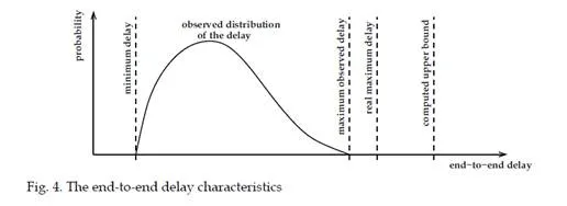
Thanks to the Integrated Modular Avionics concept [ARI (1991; 1997)], functions developed for civilian aircraft share computation resources. However, the continual growing number of these functions implies a huge increase in the quantity of data exchanged and thus in the number of connections between functions. Consequently, traditional ARINC 429 buses [ARI (2001)] can’t cope with the communication needs of modern aircraft. Indeed, ARINC 429 is a single-emitter bus with limited bandwidth and a huge number of buses would be required. Clearly, this is unacceptable in terms of weight and complexity.In order to cope with this problem, the AFDX (Avionics Full DupleX Switched Ethernet) [ARI (2002-2005)] was defined and has become the reference communication technology in the context of avionics. AFDX is a full duplex switched Ethernet network to which new mechanisms have been added in order to guarantee the determinism of avionic communications. This determinism has to be proved for certification reasons and an important challenge is to demonstrate that an upper bound can be determined for end-to- end communication delays.An important assumption is that all the avionics communication needs can be statically described: asynchronous multicast communication flows are identified and quantified. All these flows can be statically mapped on the network of AFDX switches. For a given flow, the end-to-end communication delay of a frame can be described as the sum of transmission delays on links and latencies in switches. Thanks to full duplex links characteristics, no collision can occur on links and transmission delays on links depend solely on bandwidth and frame length. But, as confluent asynchronous flows compete, on each switch output port, highly variable latencies can occur when a frame crosses a switch. Thus it is necessary to analyze these latencies in order to determine the upper bounds on end-to-end communication delays for each flow. At least three approaches have been proposed in order to compute a worst-case bound for each communication flow of the avionic applications on an AFDX network configuration. They are based on network calculus, trajectories and model checking. Such a worst-case communication delay analysis allows the comparison between the computed upper bounds and the constraints on the communication delays of each flow. Moreover it allows the scaling of the switches memory buffers in order to avoid buffer overflow and frame losses. However, communication delays measured on a real configuration are much lower than the computed upper bound. This is mainly due to the fact that rare events are difficult to observe on a real configuration in a reasonable time.
In order to better understand the real behavior of the AFDX network, a simulation model of the network is proposed as a second step. Such a simulation approach allows the calculation, on the modeled network, of the end-to-end delay for each flow, according to a representative subset of possible scenarios. Thus an end-to-end delay distribution can be obtained for each flow, leading to a better understanding of communication delays. However such an approach cannot be used for certification needs as rare events can be missed by simulation. This chapter summarizes the assumptions of the AFDX network technology and gives an overview of the different approaches which are used for the temporal analysis of such networks, i.e. the three approaches for the worst-case analysis and the simulation approach for the computation of the distributions of the end to end delays. The approaches are illustrated on a sample configuration and results on a realistic avionic configuration are shown.
Theend-to-end delay analysis of an AFDXnetwork
This section gives a short overview of an AFDX network and characterizes the end-to-end delay of a flow transmitted on such a network.
Over view of an AFDX network
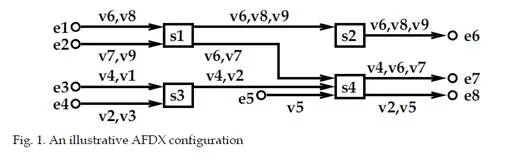
The AFDX (Avionics Full DupleX Switched Ethernet) [ARI (2002-2005)] is a switched Ethernet network taking into account avionic constraints. An illustrative example is depicted in figure 1. It is composed of four interconnected switches S1 to S4. Each switch has no input buffers on input ports and one FIFO buffer for each output port. The inputs and outputs of the network are the End Systems (e1 to e8 in Figure 1). Each end system is connected to exactly one switch port and each switch port is connected to at most one end system. Links between switches are all full duplex. The end-to-end traffic characterization is made by the definition of Virtual Links. As standardized by ARINC 664, Virtual Link (VL) is a concept of virtual communication channel. Thus it is possible to statically define all the flows (VL) which enter the network [ARI (2002-2005)]. End systems exchange Ethernet frames through VLs. Switching a frame from a transmitting to a receiving end system is based on VL. The Virtual Link defines a logical unidirectional connection from one source end system to one or more destination end systems. Coming back to the example in Figure 1, v4 is an unicast VL with path {e3 – S3 – S4 – e7}, while v6 is a multicast VL with paths {e1 – S1 – S2 – e6} and {e1 – S1 – S4 – e7}.
The routing is statically defined. Only one end system within the avionics network can be the source of one Virtual Link, (i.e. mono transmitter assumption). A VL v definition also includes the Bandwidth Allocation Gap (BAG(v)), the minimum and the maximum frame length (smin(v) and smax(v)). BAG(v) is the minimum delay between two consecutive frames of the associated VL (which actually defines a VL as a sporadic flow). VL parameters (BAG(v), smax(v)) compliance is ensured by a shaping unit at end system level and a traffic policing unit at each switch entry port (specificity of AFDX switches, compared to standard Ethernet switches). The delay incurred by the switching fabric is upper bounded by a constant value, i.e. 16 μs. A realistic AFDX configuration is presented and analyzed in section 7. It includes nearby one thousand VLs. The next paragraph characterizes the end-to-end delay of a VL transmitted on an AFDX network.
Characterizationoftheend-to-enddelayofaVL
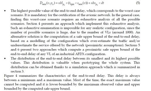
Let’s consider a path px of a VL v. The end-to-end delay D(Fv, px) of a frame Fv transmitted on px is defined by
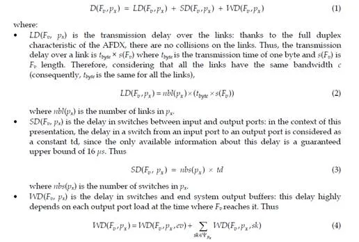
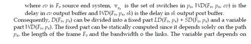
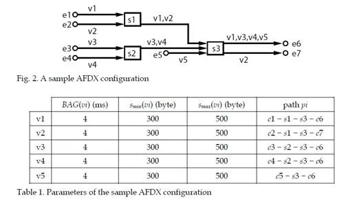
dynamic characteristics, such as the sequence of frames which are emitted by each VL (the length of each frame) and the offsets between the different VLs, i.e. the emission instant of the first frame of each VL, as it is shown by the following example.Let’s consider the AFDX configuration in figure 2. This configuration includes five unicastVLs v1. . . v5. The parameters of these VLs – their BAGs, frames sizes and paths – are given in table 1. The bandwidth of every link is 100 Mb/s (tbyte = 0,08 μs). Figure 3 exhibits three possible scenarios for the transmission of the frames of the five VLs v1. . . v5 on the network in figure 2. The switching delay td is assumed to be null. This means that SD(Fi, pi) = 0 for every frame Fi on every path pi. One single BAG of the three considered scenarios is depicted in figure 3. The analysis focuses on the end-to-end delay of the frame F1 of VL v1 (the path is p1 = e1 – s1 – s3 – e6). When the length of F1 is smax(v1) (i.e. 500 bytes), the transmission delay on the links LD(F1, p1) is 3 × (0,08 × 500) = 120 μs. When the length of F1 is smin(v1) (i.e. 300 bytes), this transmission delay LD(F1, p1) is 3 × (0,08 × 300) = 72 μs. In figure 3, the frame Fi from VL vi is denoted i.
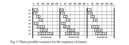
In the scenario a, each VL vi emits a frame with the maximal length smax(vi). The end-to-end delay of F1 is 160 μs. It includes the transmission on links (120 μs) and the waiting time in output port buffers (40 μs). Indeed, F1 waits for frame F2 in switch s1 and it waits for frame F3 in switch s3. In the scenario b, the frames are generated at the same instants as in the scenario a, but the length of the frame F1 of VL v1 is now 300 bytes. The end-to-end delay of F1 is now 107 μs. It includes the transmissions on links (72 μs) and the waiting time in the output port buffer in switch s3 (35 μs). The scenarios a and b show that the length of a given frame can influence its waiting delay in output port buffers. In the scenario c, v1, v2, v3 and v4 generate a frame with the maximal possible length (i.e.500 bytes), while v5 does not generate a frame. The instant where the frames from v1 and v2 are generated are switched in comparison with the two previous scenarios, while these intants are not modified for v3 and v4. In this scenario c, the frame F1 of v1 does not wait in output port buffers. Consequently, its end-to-end delay is 120 μs, i.e. the transmission time on links. This scenario shows that, for a given VL, its offset to the other VLs and the emission or non emission of frames by the other VLs influence its end-to-end delay. The end-to-end delay analysis of a path px of a VL v has to take into account all the possible scenarios. This analysis should determine the following characteristics of this end-to-end delay.
• The smallest possible value of the end-to-end delay, which corresponds to the scenarios where the VL v emits a frame with minimal length smin(v) which never waits in output ports. This smallest possible value is denoted Dmin(v, px) and it is computed from equations 1, 2 and 3:
The simulation approach for the distribution of end-to-end delays
A simulation scenario is characterized by the sequence of frames emitted by each VL and the offsets between the different VLs. It has been previously noted that a typical AFDX network includes around 1000 VLs. Clearly, this leads to a huge set of possible scenarios from which it is difficult to extract a representative subset. The resulting challenge is, for each VL path, to focus on the part of the network that is relevant for this path’s end-to-end delay distribution in order to reduce the simulation space. This is a mandatory requirement for the simulation approach. It is fulfilled by means of the VLs taxonomy that is presented in the next section.
A taxonomy ofVLs
The basic idea of the taxonomy is that, given a path px of a VL vx, the other VLs do not have the same level of influence on it. For example, a vx frame can wait for the end of transmission of another frame only if the latter shares at least one output port with px. The application of this idea is to focus the simulation on the VLs that influence the end-to-end delay distribution of vx frames.
The taxonomy is illustrated considering the unicast VL vx in figure 5. Its path px is e3-s3-s4-e8. The paths or portions of paths of other VLs of this AFDX configuration can be divided into three classes [Charara, Scharbarg & Fraboul (2006)], as depicted in figure 5.
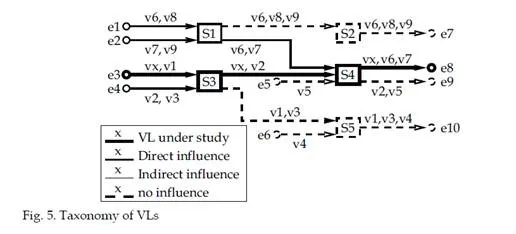
Class DI (Direct Influence) contains all the paths that share at least one output buffer with px, truncated after the last output buffer shared with px. In figure 5, it contains the whole VL v7, path e1 – s1 – s4 – e8 of v6 and sub-paths e3 – s3 and e4 – s3 – s4 of v1 and v2 respectively.
• Class II (Indirect Influence) contains all the paths or portions of paths that share no
output buffer with px, but at least one output buffer with a DI or an I I path. In figure 5, sub-paths e1 – s1 of v8, e2 – s1 of v9 and e4 – s3 of v3 are classed as indirect influence portions of VL paths.
• Class NI (No influence) contains all the paths or portions of paths that are not in class DI or class II. It contains all links
represented with dashed lines in figure 5.
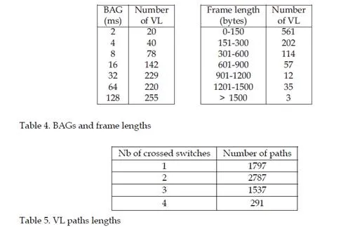
In this illustrative example containing ten VLs overall, classes DI and II each contain four and three VLs respectively. Figure 6 shows the partitioning between classes DI, II and NI for each VL path in a realistic network including 1000 VLs and 6400 paths. The continuous and dashed lines respectively give the number of VLs in class DI for each path and the number of VLs in classes DI or II. In this industrial network, on average, a VL path has 150, 650 and 200 DI, II and NI VLs respectively.
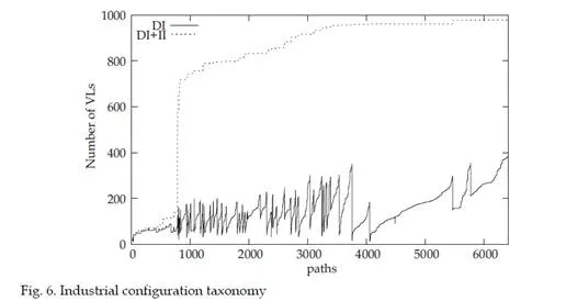
Considering this VL classification, VLs in class NI clearly have no impact on the end to end delay of their associated path px. Thus, VLs in class NI will not be considered in the definition of a scenario for a px end-to-end delay analysis. For the network analyzed in figure 6, this leads to a drastic reduction of the simulation space for approximately 800 VLs paths (each scenario includes less than 150 VLs instead of nearby 1000). Unfortunately, this reduction is quite poor for the 5600 remaining VLs paths (each scenario includes an average of 800 Vls). In order to obtain a larger reduction of the simulation space, the VL classification has to be exploited more effectively. The main idea concerns VLs in class II. They could be ignored in the definition of a scenario for a px end-to-end delay analysis provided they have no influence on px end-to-end delay distribution. The next section studies the effective influence of VLs in class II.
Effective influence of VLsin classII
The influence of a VL in class II on px is illustrated with the example depicted in figure 7. It includes one switch s1, four end systems e1, . . . , e4 and three VLs vx, v1 and v2. These three VLs have identical BAGs and frame lengths. Using the taxonomy presented in section 3.1, unicast VL vx is directly influenced by v1 (class DI) and indirectly influenced by v2 (class I I). Depending on the scenario (phasings for vx, v1 and v2), v2 can have an influence on the vx end-to-end delay by modifying the v1 arrival time at the switch s1 output port. The three possible cases are illustrated in figure 8, considering three scenarios. For each of them, figure 8 shows the modification of the vx end-to-end delay due to v2 frames. For the three scenarios, v1 and v2 are ready for transmission simultaneously and each v2 frame is arbitrarily transmitted before the corresponding v1 frame. Thus, the non-transmission of a v2 frame advances the arrival time of the corresponding v1 frame at the switch s1 output port. In scenario a in figure 8, this leads to a shorter vx end-to-end delay because it allows the v1 frame to complete transmission on the s1 – e3 link before the arrival of the vx frame at the s1 output port. Conversely, it leads to a longer vx end-to-end delay in scenario b, because the arrival order of the vx and v1 frames at the s1 output port is inverted and consequently, the vx frame has to wait. Finally, the non-transmission has no influence in scenario c, because the vx frame arrives before the v1 one in both cases and as a result never waits
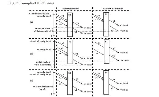
Thus, depending on the application scenario, v2 frames can shorten, lengthen or have no influence on vx end-to-end delays. However, it remains to be seen if VLs in class II (e.g. v2) modify the end-to-end delay distribution of px, their associated VL path.
In order to answer this question, every possible VL path must be examined. The basic idea is to determine, for each VL path, the end-to-end delay distributions considering first, that VLs in class II are present, and second, that they are not present. The goal is to determine whether VLs in class II modify the end-to-end delay distributions (there is at least one VL path for which the two obtained distributions are different) or not (such a VL path does not exist). In the latter case, VLs in class II do not have to be taken into account when determining end-to-end delay distributions. End-to-end delay distributions are obtained using a simulation approach. The simulation process is detailed in [Scharbarg et al. (2009)]. It considers all the possible kinds of VLs of a typical industrial AFDX configuration. For each considered VL, it compares the distribution of end-to-end delays obtained, first when VLs in class II are transmitted, second when VLs in class II are not transmitted. The two obtained distributions are the same for all the tested VLs. Thus the conclusion is that VLs in class II do not have to be taken into consideration for the computation of vx end-to-end delay distribution.
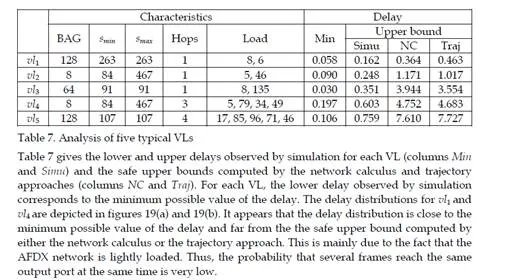
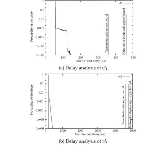
The resulting reduced simulation space makes it possible to determine an experimental probabilistic upper bound for every VL path in a realistic network. The simulation process considers a specific model for each VL path. Since an industrial network configuration includes more than 6000 paths, this leads to a heavy simulation process. A mean of speeding up this process has been presented in [Scharbarg & Fraboul (2007); Scharbarg et al. (2009)]. It consists in building a simplified model for each VL path. Such a model is depicted in Figure 9. It corresponds to a VL path which crosses two switches. The set of componants (switches and end systems) leading to each input port of a switch crossed by the path is modeled by one end system which emits all the VLs crossing this input port. It has been shown in [Scharbarg & Fraboul (2007); Scharbarg et al. (2009)] that this simplification does not modify the computed end-to-end delay distribution.
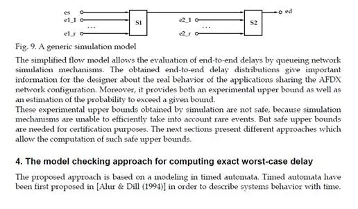
This section first gives a brief overview of timed automata. Then, the modeling of the AFDX network is presented. Finally, the verification process which computes the exact end-to-end delay upper bound is described and applied to the sample configuration in Figure 2.
Overviewoftimedautomata
A timed automaton is a finite automaton with a set of clocks, i.e. real and positive variables increasing uniformly with time. Transitions labels can be:
• a guard, i.e. a condition on clock values,
• actions,
• updates, which assign new value to clocks.
The composition of timed automata is obtained by a synchronous product. Each action a executed by a first timed automaton corresponds to an action with the same name a executed in parallel by a second timed automaton. In other words, a transition which executes the action a can be fired only if another transition labeled a is possible. The two transitions are performed simultaneously. Thus communication uses the rendez-vous mechanism. Performing transitions requires no time. Conversely, time can run in nodes. Each node is labeled by an invariant, that is a boolean condition on clocks. The node occupation is dependent of this invariant: the node is occupied if the invariant is true. Several extensions of timed automata have been proposed. One of these extensions is timed automata with shared integer variables. The principle consists in defining a set of integer variables which are shared by different timed automata. Consequently, the values of these variables can be consulted and updated by the different timed automata [Larsen et al. (1997); Burgueño Arjona (1998)]. A system modelled with timed automata can be verified using a reachability analysis which is performed by model-checking. It consists in encoding each property in terms of the reachability of a given node of one of the automata. So, a property is verified by the reachability of the associated node if and only if this node is reachable from an initial configuration. Reachability is decidable and algorithms exist [Larsen et al. (1997)]. In the general case, reachability analysis is undecidable on timed automata with shared integer variables. In the particular case where the shared variables are represented by nodes of a timed automata, the reachability analysis is decidable. The approach considered in this paper is based on timed automata with shared integer variables which are represented by nodes of a timed automaton. The modeling of the AFDX with timed automata is now presented.
The modeling of an AFDX network
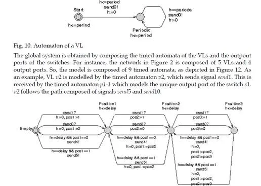
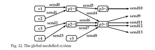
The modeling of an AFDX network considers an automaton for each VL and an automaton for each output port of a switch. Figure 10 depicts the timed automaton of a VL with a BAG equal to period. This automaton sends a first message sendi (send0 in the example) delayed by a duration between 0 and period, and then sends periodically a new message sendi (the period is equal to the BAG of the VL, i.e. period). So, this automaton models a periodic VL with an offset between 0 and its BAG. Figure 11 shows an example of an output port of a switch. Each node of the automaton models a location in the FIFO queue associated to the port. Consequently, the number of nodes of the automaton equals the size of the queue (3 in the example of Figure 11). Each transition from a node Positioni to a node Positioni+1 of the automaton models the arrival of one frame at the transmit port while each transition from a node Positioni+1 to a node Postioni models the end of the transmission from this port. The automaton of the Figure 11 considers two flows (i.e. two VLs) received using signals send0 and send1 and transmitted using signals send4 and send5, corresponding respectively to send0 and send1. delay is the transmission time of the frame. In the considered example application, all the frames have the same length. pos1, pos2 and pos3 indicate the flows (0 or 1) corresponding to the frames waiting in each position of the queue.
The computation of the exact worst-case end-to-end delay
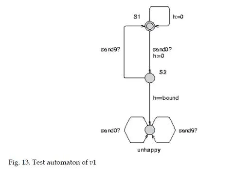
Using the test automaton method [Burgueño Arjona (1998); Bérard et al. (2001)], the worst case end-to-end delay of each VL is obtained from the model previously described. The test automaton corresponding to the VL v1 is depicted in Figure 13. This automaton models the property “delay of v1 is less than bound”. By receiving signal send0, it evolves to the node s2. Then the signal send9 is waited (transmission of v1 from the output port of the switch s3, see Figure 12). If this signal is not received before the delay of bound, the automaton evolves to the node reject. This behaviour corresponds to a scenario for which the transmission delay of v1 is greater than bound. So, the analysis consists in finding the lowest value of bound for which the node reject is reached. This value is the maximum end-to-end delay.
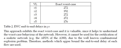
To verify the property, we use the model-checker UPPAAL. The calculation takes less than 1s on a Linux station with a Pentium 4 processor and 2GB of memory size. The exact worst case end-to-end delays obtained for each VLs in the Figure 2 are given in table 2
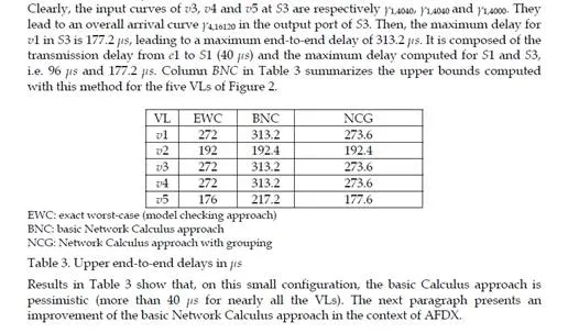
Optimizing the Network Calculus approach with grouping
The pessimism observed in Table 3 is partly due to the fact that the basic Network Calculus approach does not take into account the property that packets of different flows sharing a link cannot be transmitted at the same time on this link (they are serialized). Consequently, the burst considered in the overall input curves of the basic Network Calculus approach can never happen, as soon as at least two flows share the same link. This problem is different from the classical “pay burst only once” case described in [Le Boudec & Thiran (2001)]. Indeed, the objective of “pay burst only once” is to aggregate successive switches in order to give an optimized aggregated service curve. The aggregation of nodes is not possible in our case, since flows can join and leave a path at any switch of the network.On the example in Figure 2, the input curve of the output port of S3 shared by v1, v3, v4 and v5 is ┛4,16120. The maximum burst (16120 bits) corresponds to the case where four packets – one for each VL – arrive at the same time in the output port. This is definitely impossible, since v3 and v4 share the same link. The grouping technique integrates this serialization.
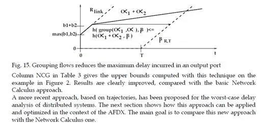
It proceeds in two steps. First, the overall arrival curve is computed for each link. It is the minimum between, on the one hand the sum of the arrival curves of all the flows sharing the considered link, on the other hand the curve bounding the burst to the maximum burst among the curves of the different flows sharing the link and the rate to the rate of the link. This first step is illustrated in Figure 15 for a link shared by two flows with arrival curve
| 1 1 |
| 2 2 |
γr,b and γr,bIn the second step, the curves obtained for the different links are added.
The gain obtained with this technique is due to the reduction of the maximum burst.
AFDX worst –case delay analysis with the Trajectory approach
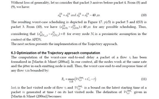
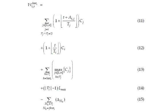
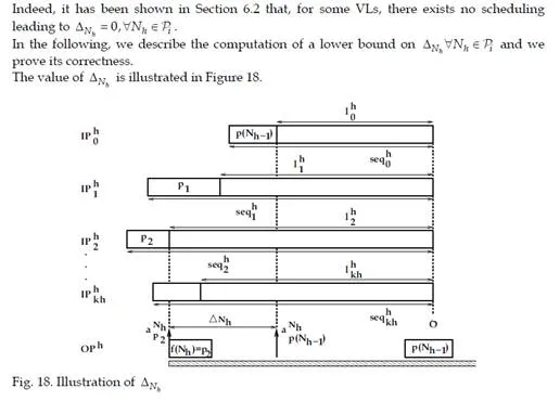
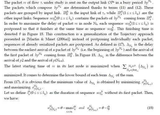
The Trajectory approach [Martin (2004); Martin & Minet (2006a); Migge (1999)] has been developed to get deterministic upper bounds on end-to-end response time in distributed systems. This approach considers a set of sporadic flows with no assumption concerning the arrival time of packets. The principle of the application of the Trajectory approach to the AFDX has been presented in [Bauer et al. (2009a)]. The improvement of the approach has been proposed in [Bauer et al. (2009b)]. Main features of the Trajectory approach applied to AFDX are summarized and illustrated in Sections 6.1 and 6.2. The proof of the optimization of the Trajectory approach computation is presented in Section 6.3.
The main features of the Trajectory approach
The approach developed for the analysis of the AFDX considers the results from [Martin & Minet (2006a)]. A distributed system is composed of a set of interconnected processing nodes. Each flow crossing this system follows a static path which is an ordered sequence of nodes. The Trajectory approach assumes, with regards to any flow τi following path Pi, that any flow j following path Pj, with Pj ≠ Pi and Pj ∩ PI ≠ ∅, never visits a node of path Pi after having left this path.Flows are scheduled with a FIFO algorithm in every visited node. Each flow τi has a minimum inter-arrival time between two consecutive packets at ingress node, denoted Ti, a maximum release jitter at the ingress node denoted Ji, an end-to-end deadline Di that is the
| C |
| i |
maximum end-to-end response time acceptable and a maximum processing time hon each node Nh, with Nh ∈ Pi. The transmission time of any packet on any link between nodes has known lower and upper bounds Lmin and Lmax and there are neither collisions nor packet losses on links. The end-to- end response time of a packet is the sum of the times spent in each crossed node and the transmission delays on links. The transmission delays on links are upper bounded by Lmax. The time spent by a packet m in a node Nh depends on the pending packets in Nh at the arrival time of m in Nh. The problem is then to upper bound the overall time spent in the visited nodes.
The solution proposed by the Trajectory approach is based on the busy period concept. A busy period of level L is an interval [t, t’) such that t and t’ are both idle times of level L and there is no idle time of level L in (t, t’). An idle time t of level L is a time such as all packets with priority greater than or equal to L generated before t have been processed at time t. With FIFO scheduling, no packet from the busy period of level corresponding to the priority of m could have arrived after m on the considered node.The Trajectory approach considers a packet m from flow τi generated at time t. It identifies the busy period and the packets impacting its end-to-end delay on all the nodes visited by m (starting from the last visited node backward to the ingress node). This decomposition enables the computation of the latest starting time of m on its last node. This starting time can be computed recursively and leads to the worst case end-to-end response time of the flow τi. This computation will be illustrated in the context of AFDX.
The elements of the system considered in the Trajectory approach are instantiated in the following way in the context of AFDX:
• each node of the system corresponds to an AFDX switch output port, including the output link,
• each link of the system corresponds to the switching fabric,
• each flow corresponds to a VL path.
The assumptions of the Trajectory approach are verified by the AFDX (see Section 2.1). Indeed, switch output ports implement FIFO service discipline. The switching fabric delay is upper bounded by a constant value (16 μs), thus L = Lmin = Lmax = 16 μs. There are no collisions nor packet loss on AFDX networks. The routing of the VLs is statically defined. VL parameters match the definition of sporadic flows in the following manner:
Ti = BAG,
| C |
| i |
| i |
h= smax/R, Ji = 0. Since all the AFDX ports work at the same rate R = 100Mb/s, Ch= Ci =
smax/R for every node h in the network.
Illustration on a sample AFDX configuration
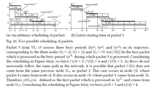
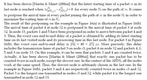
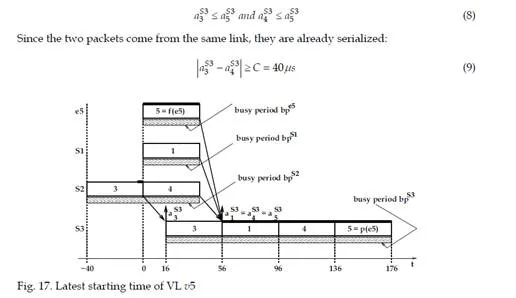
Let us consider the sample AFDX configuration depicted in Figure 2. Figure 16(a) shows an arbitrary scheduling of the packets, which are identified by their VL numbers (e.g. packet 3 is a packet from VL v3). The scheduling in Figure 16(a) focuses on packet 3. The arrival time
| m |
of a packet m in a node Nh is denoted aNh . Time origin is arbitrarily chosen as the arrival time of packet 3 in node e3. The processing time of a packet in a node is 40 μs. It corresponds to the transmission time of the packet on a link. The delay between the end of the processing of a packet by a node and its arrival in the next node corresponds to the 16 μs switch factory delay. Due to the FIFO policy, packet 3 is delayed by packet 4 in S2. In node S3, packet 5 is delayed by packet 1 and delays packet 4, which delays packet 3.
Conclusion
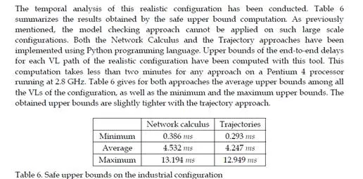
This chapter gives an overview of the temporal analysis of switched Ethernet avionic networks. Today, three approaches exist for the computation of a safe upper bound of the end-to-end delay of each flow transmitted on the avionic network. The first approach is based on model checking and allows the computation of the exact worst-case delay of each flow, but it is limited to small configurations, due to the combinatory explosion problem. The two other approaches are based on trajectories and network calculus and allow the computation of a safe upper bound of the end-to-end delay, which is most of the time larger than the exact worst-case, due to the pessimistic assumptions made by the two approaches. Nevertheless, these two approaches can be applied to industrial configurations. The computation of a safe upper bound is complemented by the evaluation of the end-to-end delay distribution, thanks to a simulation approach.The worst-case analysis approaches presented in this paper consider a set of sporadic flows with no assumption concerning the arrival time of packets. This does not take into account the scheduling of the flows which are emitted by the same component. This scheduling could be integrated in the modeling by the mean of assumptions on the relative arrival time of packets, as it has been done in the automotive context [Grenier et al. (2008)]. The integration of this scheduling in the modeling of flows should distribute temporally the transmission of packets and very likely reduce the waiting time of packets in output buffers. Moreover, the sporadic characteristic of avionics flows could be taken into account with the help of a probabilistic modeling, as it has been proposed for the a periodic traffic in the automotive context [Khan et al. (2009)]. This leads to a probabilistic analysis of the worst case delay of flows. Such an analysis has been proposed [Scharbarg et al. (2009)], based on a stochastic Network Calculus approach [Vojnović & Le Boudec (2002; 2003)].For future aircraft, the addition of other type of flows (audio, video, best-effort, . . .) on the AFDX network is envisioned. These different flows have different timing constraints and criticity levels. Thus, it is necessary to differentiate them and the FIFO policy on switch output ports is not suitable. Thus, it is necessary to consider other service disciplines, such as static priority queueing or weighted fair queueing [Parekh & Gallager (1993)]. The introduction of static priority queueing in the stochastic Network Calculus approach has been presented in [Ridouard et al. (2008)]. The Trajectory approach is promising for handling heterogeneous flows needing QoS aware servicing policies at switches level [Martin & Minet (2006a;b)].