When mechanical engineers design automobiles, aircraft, rockets, and other vehicles, they generally need to know the drag force FD that will resist high speed motion through the air or water . In this section, we will discuss the drag force and a related quantity that is known as the coefficient of drag, denoted by CD. That parameter quantifies the extent to which an object is streamlined, and it is used to calculate the amount of resistance that an object will experience as it moves through a fluid (or as fluid flows around it). Whereas buoyancy forces develop even in stationary fluids, the drag force and the lift force arise from the relative motion between a fluid and a solid object. The general behavior of moving fluids and the motions of objects through them define the field of mechanical engineering known as fluid dynamics.
Drag Force Equation
For values of the Reynolds number that can encompass either laminar or turbulent flow, the magnitude of the drag force is determined by the equation
where rho – (ρ) is the fluid’s density, and the area A of the object facing the flowing fluid is called the frontal area. In general, the magnitude of the drag force increases with the area that impinges on the fluid. The drag force also increases with the density of the fluid (for instance, air versus water), and it grows with the square of the speed.

Figure : The Space Shuttle Orbiter touches down at the Kennedy Space Center. The aerodynamic design of the Orbiter was a compromise for operation over a wide range of conditions: ascent through the relatively dense lower atmosphere, hypersonic reentry in the upper atmosphere, and un-powered gliding flight to touchdown. In that latter phase, the Orbiter was described, only partially in jest, as a flying brick.
If all other factors remain the same, the drag force exerted on an automobile going twice as fast as another would be four times greater. The drag coefficient is a single numerical value that represents the complex dependency of the drag force on the shape of an object and its orientation relative to the flowing fluid. Equation stated above is valid for any object, regardless of whether the flow is laminar or turbulent, provided that one knows the numerical value for the coefficient of drag. However, mathematical equations for CD are available only for idealized geometries (such as spheres, flat plates, and cylinders) and restricted conditions (such as a low Reynolds number). In many cases, mechanical engineers must still obtain practical results, even for situations where the coefficient of drag can’t be described mathematically. In such cases, engineers rely on a combination of laboratory experiments and computer simulations. Through such methods, numerical values for the drag coefficient have been tabulated in the engineering literature for a wide range of applications. For instance, a relatively buff sport-utility vehicle has a larger coefficient of drag (and a larger frontal area as well) than a sports car. By using the values of CD and A in this table, as well as other published data, the drag force can be calculated using Equation above. To illustrate, Figure below depicts the drag force that acts on a sphere as fluid flows around it (or the force that would develop as the sphere moves through the fluid). Regardless of whether the sphere or fluid is moving, the relative velocity v between the two is the same. The sphere’s frontal area as seen by the fluid is A = ¼Πd^2. In fact, the interaction between a sphere and a fluid has important engineering applications to devices that deliver medicine through aerosol sprays, to the motion of pollutant particles in the atmosphere, and to the modeling of raindrops and hailstones in storms. Graph below shows how the drag coefficient for a smooth sphere changes as a function of the Reynolds number over the range
0.1 < Re < 100,000. At the higher values, say 1000 < Re < 100,000, the drag coefficient is nearly constant at the value CD ~ 0.5.
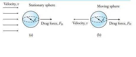
Figure: The drag force depends on the relative velocity between a fluid and an object. (a) Fluid flows past a stationary sphere and creates the drag force FD. (b) The fluid is now stationary and the sphere moves through it
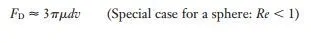
When it is combined with the graph below, this equation can be used to calculate the drag force acting on a sphere. When Re is very low, so that the low is smooth and laminar, the drag coefficient is given approximately by
This result is shown as the dotted line in the logarithmic representation of Graph. You can see that the result from above equation agrees with the more general CD curve only when the Reynolds number is less than one. This substitution of the equation into drag force equation gives the low-speed approximation for the sphere’s drag force
(Equation 6.16)
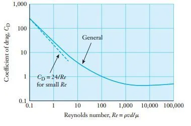
Graph : Dependence of the drag coefficient for a smooth sphere on the Reynolds number (solid line), and the value predicted for low Re from Equation (dashed line)
Although this result is valid only for low speeds, you can see how the magnitude of FD increases in relation to speed, the fluid’s viscosity, and the sphere’s diameter. Experiments show that Equation (6.16) starts to underestimate the drag force as the Reynolds number grows. Because the fundamental character of a fluid’s flow pattern changes from laminar to turbulent with Re (Figure 6.14), Equations (6.15) and (6.16) are applicable only when Re is less than one and the flow is unmistakably laminar. When those equations are used in any calculation, you should be sure to verify that the condition Re < 1 is met.

